Module 5: Visualization with Matplotlib & Leafmap¶
Learning Goals¶
- Create static maps with matplotlib
- Plot multiple GeoPandas layers
- Introduction to leafmap for interactive mapping
- Change basemaps and add layers
- Add popups and interactive elements
- Export and print maps
Matplotlib¶
Matplotlib is Python’s most widely used library for drawing charts and maps as static pictures—line graphs, scatter plots, histograms, bar charts, and (with a little help from GeoPandas) maps with coastlines, regions, and points.
Think of it in three plain ideas:
- Figure and axes — You usually start with
fig, ax = plt.subplots(...). The figure is the whole canvas (the window or image file). The axes (ax) is the drawing area where you plot: titles, labels, limits, and the actual geometry all attach toax. pyplot(plt) — Thematplotlib.pyplotmodule is the simple, step-by-step interface you’ll see in tutorials:plt.plot,plt.show,plt.savefig. Under the hood it still uses figures and axes;plt.subplotsis just a convenient way to create them.- Static output — Matplotlib is built for non-interactive figures: you run code, get an image (on screen or PNG/PDF). For pan/zoom maps in the browser, use Leafmap (§ 2. Leafmap below); Matplotlib stays the workhorse for publication-style and notebook maps.
You do not need to memorize every function at once. The patterns in this module—plot, scatter, colors, legends, GeoDataFrame.plot(ax=...)—repeat across most geospatial visualization workflows.
Install the libraries used in the Matplotlib examples below (terminal, or a notebook cell with !pip):
Below are small Matplotlib + rasterio recipes for a single-band GeoTIFF (paths point at the bundled /content/Tiff_1.tif; change path if your file lives elsewhere). Each block is meant to copy into a notebook as a starting point.
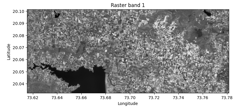
Display raster image¶
imshow draws the 2D array as a grid of colored cells. Pass extent=[left, right, bottom, top] from src.bounds so the image lines up with map coordinates (here lon/lat for EPSG:4326). origin="upper" matches typical raster row order (north at the top).
import matplotlib.pyplot as plt
import rasterio

path = "/content/Tiff_1.tif"
with rasterio.open(path) as src:
    band = src.read(1)
    bounds = src.bounds  # left, bottom, right, top

extent = [bounds.left, bounds.right, bounds.bottom, bounds.top]
fig, ax = plt.subplots(figsize=(8, 6))
ax.imshow(band, cmap="gray", extent=extent, origin="upper")
ax.set_xlabel("Longitude")
ax.set_ylabel("Latitude")
ax.set_title("Raster band 1")
plt.tight_layout()
plt.show()
Example output:
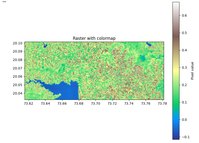
Apply colormap¶
A colormap maps numeric cell values to colors. cmap picks the palette (try terrain, viridis, RdYlGn). Add plt.colorbar so readers can relate color to value; use vmin / vmax to stretch contrast when needed.
import matplotlib.pyplot as plt
import rasterio

path = "/content/Tiff_1.tif"
with rasterio.open(path) as src:
    band = src.read(1).astype(float)
    b = src.bounds
    extent = [b.left, b.right, b.bottom, b.top]

fig, ax = plt.subplots(figsize=(8, 6))
im = ax.imshow(band, cmap="terrain", extent=extent, origin="upper")
plt.colorbar(im, ax=ax, label="Pixel value")
ax.set_title("Raster with colormap")
plt.tight_layout()
plt.show()
Example output:
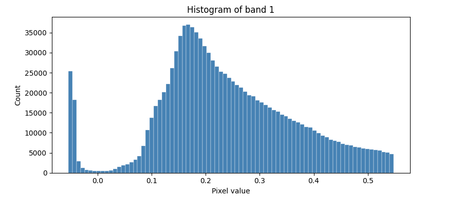
Histogram (pixel distribution)¶
A histogram counts how many pixels fall into value bins. It summarizes the whole band (distribution, skew, outliers). Use flatten() on the 2D array; np.nanpercentile helps choose range=(lo, hi) so a few extreme pixels do not squash the bars.
import matplotlib.pyplot as plt
import numpy as np
import rasterio

path = "/content/Tiff_1.tif"
with rasterio.open(path) as src:
    arr = src.read(1).astype(float)

lo, hi = np.nanpercentile(arr, [2, 98])
fig, ax = plt.subplots(figsize=(8, 4))
ax.hist(arr.flatten(), bins=80, range=(lo, hi), color="steelblue", edgecolor="white", linewidth=0.3)
ax.set_xlabel("Pixel value")
ax.set_ylabel("Count")
ax.set_title("Histogram of band 1")
plt.tight_layout()
plt.show()
Example output:
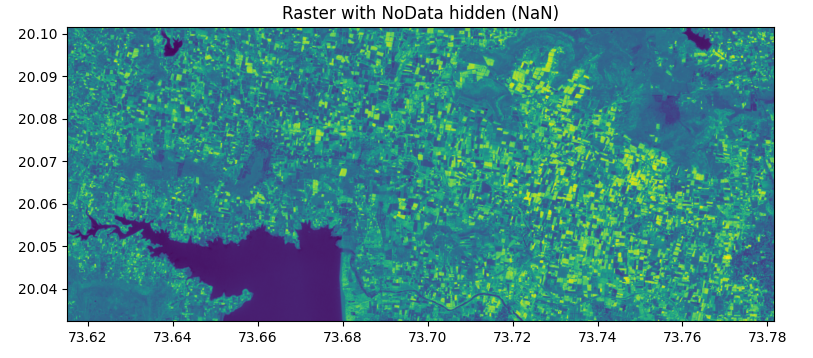
Remove NoData / black pixels¶
Rasters often mark missing cells with a NoData sentinel or they appear as a flat black edge. For plotting, replace those values with np.nan so imshow does not paint them, or mask them before hist. Always read src.nodata from the file when it is set.
import matplotlib.pyplot as plt
import numpy as np
import rasterio

path = "/content/Tiff_1.tif"
with rasterio.open(path) as src:
    band = src.read(1).astype(float)
    nd = src.nodata
    b = src.bounds
    extent = [b.left, b.right, b.bottom, b.top]

if nd is not None:
    band = np.where(band == nd, np.nan, band)

fig, ax = plt.subplots(figsize=(8, 6))
ax.imshow(band, cmap="viridis", extent=extent, origin="upper")
ax.set_title("Raster with NoData hidden (NaN)")
plt.tight_layout()
plt.show()
Example output:
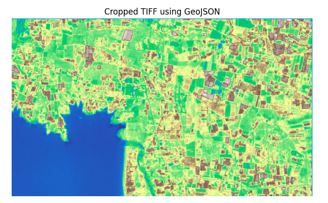
Zoom / crop view¶
Zooming only changes what Matplotlib shows: call set_xlim and set_ylim on the same full raster. Cropping loads a smaller window with from_bounds, which saves memory on large GeoTIFFs. Use plotting_extent so imshow’s extent matches the window’s georeferencing.
import matplotlib.pyplot as plt
import rasterio
from rasterio.mask import mask
import json

path = "/content/Tiff_1.tif"

# Your GeoJSON polygon
geojson = {
  "type": "FeatureCollection",
  "features": [
    {
      "type": "Feature",
      "properties": {},
      "geometry": {
        "coordinates": [[
          [73.66053541139414, 20.069929645956293],
          [73.66053541139414, 20.039907375765722],
          [73.71140637660173, 20.039907375765722],
          [73.71140637660173, 20.069929645956293],
          [73.66053541139414, 20.069929645956293]
        ]],
        "type": "Polygon"
      }
    }
  ]
}

# Extract geometry
shapes = [feature["geometry"] for feature in geojson["features"]]

with rasterio.open(path) as src:
    cropped, transform = mask(src, shapes, crop=True)

# Plot
plt.figure(figsize=(8, 6))
plt.imshow(cropped[0], cmap="terrain")
plt.title("Cropped TIFF using GeoJSON")
plt.axis("off")
plt.show()
Example output:
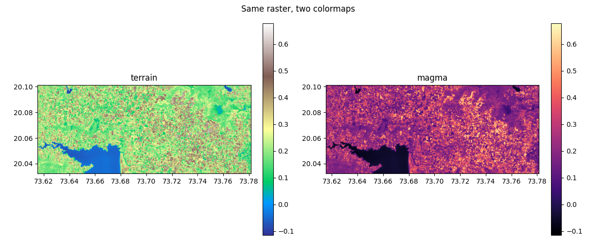
Multiple subplots¶
plt.subplots(nrows, ncols) returns a grid of axes so you can compare the same band with different cmaps, or histogram + map, side by side. Keep extent consistent across map panels so geography aligns.
import matplotlib.pyplot as plt
import numpy as np
import rasterio

path = "/content/Tiff_1.tif"
with rasterio.open(path) as src:
    band = src.read(1).astype(float)
    b = src.bounds
    extent = [b.left, b.right, b.bottom, b.top]

fig, axes = plt.subplots(1, 2, figsize=(12, 5))
im0 = axes[0].imshow(band, cmap="terrain", extent=extent, origin="upper")
axes[0].set_title("terrain")
plt.colorbar(im0, ax=axes[0], fraction=0.046)

im1 = axes[1].imshow(band, cmap="magma", extent=extent, origin="upper")
axes[1].set_title("magma")
plt.colorbar(im1, ax=axes[1], fraction=0.046)

plt.suptitle("Same raster, two colormaps")
plt.tight_layout()
plt.show()
Example output:
2. Leafmap¶
Leafmap is a Python library for interactive maps in notebooks (Jupyter, Colab, VS Code). It sits on top of ipyleaflet and folium (depending on backend) and talks to Leaflet in the browser: you get pan, zoom, layer toggles, and popups without building JavaScript yourself. Use it when you want to explore data on a basemap, compare layers, or share a map as HTML—after Matplotlib or GeoPandas when you need a live map rather than a static figure.
Paths below use assets/... as in this repo; on Colab, point at /content/... instead. End a cell with m to display the widget (or use your environment’s equivalent).
Install Leafmap and, if you use add_raster on local GeoTIFFs, localtileserver (see the raster subsection below):
Create map¶
A leafmap.Map is the canvas: center=[latitude, longitude] (lat first) and zoom set the initial view; height sizes the widget in the notebook.
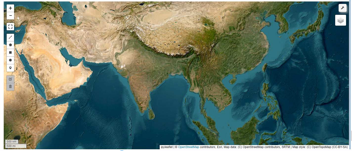
Add basemap¶
add_basemap stacks a named tile layer (streets, imagery, terrain). Discover names with leafmap.basemaps.keys(). Add add_layer_control() so readers can turn layers on or off.
import leafmap

m = leafmap.Map(center=[20.07, 73.70], zoom=10)
m.add_basemap("Esri.WorldImagery")
m.add_basemap("OpenTopoMap")
m.add_layer_control()
m
Example output:
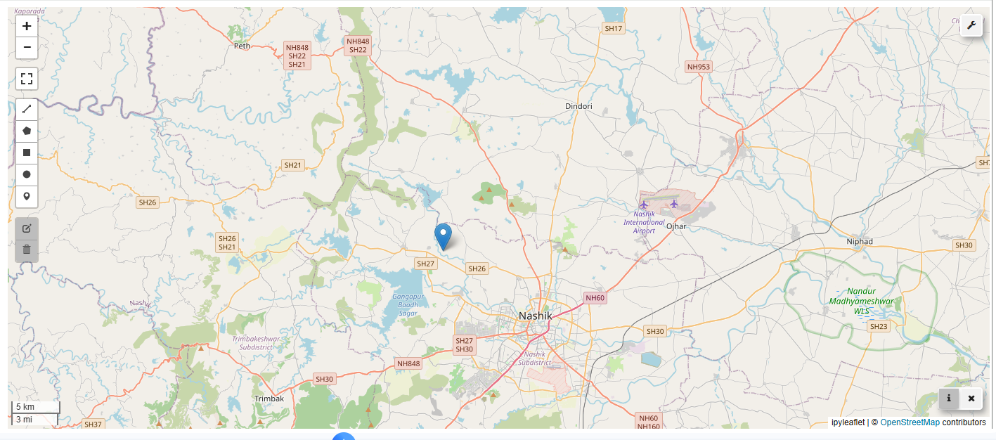
Add marker¶
add_markers drops one or more pin or circle markers at [lat, lon] positions (a list of lists for many points). Use shape, color, and popup arguments to customize when your leafmap version supports them.
import leafmap

m = leafmap.Map(center=[20.07, 73.70], zoom=11)
m.add_markers(markers=[[20.07, 73.70]], shape="marker")
m
Example output:
Add GeoJSON¶
add_geojson loads vector features from a URL or file path. Set layer_name for the layer list; optional styling arguments depend on your leafmap version (see add vector).
import leafmap

m = leafmap.Map(center=[20, 78], zoom=5, height="520px")

# GeoJSON as Python dict
geojson_data = {
    "type": "FeatureCollection",
    "features": [
        {
            "type": "Feature",
            "properties": {"name": "My Area"},
            "geometry": {
                "type": "Polygon",
                "coordinates": [[
                    [73.71, 20.09],
                    [73.69, 20.07],
                    [73.72, 20.06],
                    [73.73, 20.08],
                    [73.71, 20.09]
                ]]
            }
        }
    ]
}

# Add directly (no file needed)
m.add_geojson(geojson_data, layer_name="GeoJSON Area")

m.add_layer_control()
m
Example output:
Export map¶
to_html writes a standalone HTML file you can open in a browser or host on the web. Build the map first, then export; very heavy layers can make large files.
import leafmap.foliumap as leafmap   # ✅ use folium backend

m = leafmap.Map(center=[20.07, 73.70], zoom=10)
m.add_basemap("CartoDB.Positron")

# ✅ correct method
m.add_marker(location=[20.07, 73.70])

m.to_html("leafmap_export.html")

print("Saved leafmap_export.html")
Basics assignment: Matplotlib & Leafmap¶
These tasks recap the core visualization patterns in this module: make a clear static figure with Matplotlib, then build an interactive map with Leafmap. Use the bundled raster assets/tiff/Tiff_1.tif (and the example screenshots in docs/assets/) to keep the setup simple.
Where to run these
- In notebooks, end a Leafmap cell with
mto display the map widget. - If you run in Colab, your files may live under
/content/instead ofassets/.
-
Display a raster — Use
rasterio.open(...)+imshowto display band 1 ofassets/tiff/Tiff_1.tifwith anextentfromsrc.bounds. -
Colormap + legend — Re-plot the same band with a different
cmap(e.g.terrain) and add acolorbar. -
Histogram — Plot the pixel distribution (ignore NoData if present). Write one sentence describing what the histogram shape suggests (e.g. many mid-values vs many extremes).
-
Mask NoData — Convert
src.nodatavalues tonp.nanand confirm your map no longer paints those pixels. -
Crop a view — Read a window with
from_bounds(...)and plot only that area (a “zoomed-in” raster view). -
Leafmap basemap — Create
leafmap.Map(...), add at least one basemap, and enableadd_layer_control(). -
Leafmap marker — Add a marker near your raster extent (or any location you choose) and confirm it appears at the right place.
-
Leafmap GeoJSON — Add GeoJSON (either the inline
geojson_dataexample from this module orassets/examples/example.geojson) and toggle it on/off in the layer control. -
Export — Save your final Leafmap view as HTML using
to_html("my_map.html")and open the file in a browser.
Submit your notebook (.ipynb) or script (.py) plus any exported HTML files your instructor requests.
¶
¶
Advance¶
Setting Up the Environment¶
import geopandas as gpd
import matplotlib.pyplot as plt
import numpy as np
import leafmap
import warnings
warnings.filterwarnings('ignore')

# Load sample data
import geopandas as gpd

world=gpd.read_file("/content/countries.zip")
states=gpd.read_file("/content/states.zip")
cities=gpd.read_file("/content/city.geojson")

print("=== DATA LOADED ===")
print(f"World countries: {len(world)}")
print(f"Cities: {len(cities)}")
1. Basic Plotting with Matplotlib¶
Single Layer Visualization¶
# Basic world map
fig, ax = plt.subplots(1, 1, figsize=(15, 10))

# Plot world countries
world.plot(ax=ax, color='lightblue', edgecolor='black', linewidth=0.5)

# Customize the map
ax.set_title('World Countries', fontsize=16, fontweight='bold')
ax.set_xlabel('Longitude')
ax.set_ylabel('Latitude')

# Remove axis ticks for cleaner look
ax.set_xticks([])
ax.set_yticks([])

plt.tight_layout()
plt.show()
Multiple Layer Visualization¶
# Plot multiple layers together
fig, ax = plt.subplots(1, 1, figsize=(15, 10))

# Plot countries as base layer
world.plot(ax=ax, color='lightgray', edgecolor='black', linewidth=0.3, alpha=0.7)

# Plot cities on top
cities.plot(ax=ax, color='red', markersize=20, alpha=0.8)

# Customize
ax.set_title('World Countries and Major Cities', fontsize=16, fontweight='bold')
ax.set_xlim(-180, 180)
ax.set_ylim(-60, 80)
ax.set_xticks([])
ax.set_yticks([])

plt.tight_layout()
plt.show()
Choropleth Maps¶
# Create choropleth map by population
fig, ax = plt.subplots(1, 1, figsize=(15, 10))

# Plot with population-based colors
world.plot(
    column='POP_EST',
    ax=ax,
    cmap='YlOrRd',
    edgecolor='black',
    linewidth=0.3,
    legend=True,
    legend_kwds={'label': 'Population Estimate', 'shrink': 0.8}
)

# Add cities
cities.plot(ax=ax, color='blue', markersize=15, alpha=0.7)

ax.set_title('World Population and Major Cities', fontsize=16, fontweight='bold')
ax.set_xticks([])
ax.set_yticks([])

plt.tight_layout()
plt.show()
Focused Regional Maps¶
# Focus on Europe
print("Available columns in cities:", cities.columns)
europe = world[world['REGION_UN'] == 'Europe']

# Get a list of European country names from the 'europe' GeoDataFrame
european_country_names = europe['NAME'].unique().tolist()

# Filter cities to include only those within European countries
europe_cities = cities[cities['country'].isin(european_country_names)]

fig, ax = plt.subplots(1, 1, figsize=(12, 10))

# Plot European countries
europe.plot(ax=ax, color='lightgreen', edgecolor='black', linewidth=0.5)

# Plot European cities
europe_cities.plot(ax=ax, color='red', markersize=50, alpha=0.8)

# Add city labels for major cities
major_cities = europe_cities[europe_cities['population'] > 2000000] # Use 'population' instead of 'POP_EST' for cities
for idx, city in major_cities.iterrows():
    ax.annotate(city['city'], # Use 'city' instead of 'NAME' for city labels
                (city.geometry.x, city.geometry.y),
                xytext=(5, 5), textcoords='offset points',
                fontsize=8, fontweight='bold')

ax.set_title('European Countries and Major Cities', fontsize=14, fontweight='bold')
ax.set_xlim(-25, 45)
ax.set_ylim(35, 75)

plt.tight_layout()
plt.show()
3. Changing Basemaps¶
Available Basemaps¶
# List available basemaps
print("Available basemaps:")
for basemap in leafmap.basemaps.keys():
    print(f"  - {basemap}")
Switching Basemaps¶
# Create map with different basemap
m = leafmap.Map(center=[40, -100], zoom=4)

# Add basemap selector
m.add_basemap('Esri.WorldImagery')  # Satellite imagery
m
# Try different basemaps
m = leafmap.Map(center=[40, -100], zoom=4)
m.add_basemap('CartoDB.Positron')  # Light basemap
m
# Terrain basemap
m = leafmap.Map(center=[40, -100], zoom=4)
m.add_basemap('Esri.WorldTopoMap')  # Topographic map
m
4. Adding GeoPandas Layers¶
Add Vector Data¶
# Create map and add countries
m = leafmap.Map(center=[20, 0], zoom=2)

# Add world countries
m.add_gdf(
    world,
    layer_name='Countries',
    fill_colors=['lightblue'],
    line_colors=['black'],
    line_widths=[0.5]
)

m
Add Multiple Layers¶
# Create map with multiple layers
m = leafmap.Map(center=[20, 0], zoom=2)

# Add countries layer
m.add_gdf(
    world,
    layer_name='Countries',
    fill_colors=['lightgray'],
    line_colors=['black'],
    line_widths=[0.3]
)

# Add cities layer
m.add_gdf(
    cities,
    layer_name='Cities',
    fill_colors=['red'],
    point_size=5
)

# Add layer control
m.add_layer_control()

m
Styled Layers¶
# Create styled map
m = leafmap.Map(center=[20, 0], zoom=2)

# Add countries with population-based styling
m.add_gdf(
    world,
    column='pop_est',
    layer_name='Population',
    cmap='YlOrRd',
    legend_title='Population',
    line_colors=['black'],
    line_widths=[0.3]
)

m
5. Adding Popups¶
Basic Popups¶
# Create map with popups
m = leafmap.Map(center=[20, 0], zoom=2)

# Add countries with popup information
m.add_gdf(
    world,
    layer_name='Countries',
    info_cols=['name', 'continent', 'pop_est'],  # Columns to show in popup
    fill_colors=['lightblue'],
    line_colors=['black']
)

m
Custom Popup Content¶
# Create formatted popup content
world_popup = world.copy()
world_popup['popup_info'] = world_popup.apply(
    lambda row: f"""
    <b>{row['name']}</b><br>
    Continent: {row['REGION_UN']}<br>
    Population: {row['POP_EST']:,}<br>
    GDP: ${row['gdp_md']:,.0f}M
    """, axis=1
)

m = leafmap.Map(center=[20, 0], zoom=2)

# Add with custom popup
m.add_gdf(
    world_popup,
    layer_name='Countries',
    info_cols=['popup_info'],
    fill_colors=['lightgreen'],
    line_colors=['black']
)

m
City Popups¶
# Create map with city popups
m = leafmap.Map(center=[20, 0], zoom=2)

# Add countries
m.add_gdf(
    world,
    layer_name='Countries',
    fill_colors=['lightgray'],
    line_colors=['black'],
    line_widths=[0.3]
)

# Add cities with detailed popups
m.add_gdf(
    cities,
    layer_name='Cities',
    info_cols=['name', 'country', 'pop_max'],
    fill_colors=['red'],
    point_size=8
)

m.add_layer_control()
m
6. Print and Export Maps¶
Save as HTML¶
# Create and save map
m = leafmap.Map(center=[40, -100], zoom=4)

# Add some data
m.add_gdf(
    world[world['continent'] == 'North America'],
    layer_name='North America',
    fill_colors=['lightgreen'],
    line_colors=['black']
)

# Save to HTML file
m.to_html('north_america_map.html')
print("Map saved as 'north_america_map.html'")
Save as Image¶
# Save map as PNG image
m = leafmap.Map(center=[40, -100], zoom=4)

m.add_gdf(
    world[world['continent'] == 'North America'],
    layer_name='North America',
    fill_colors=['lightblue'],
    line_colors=['black']
)

# Save as image (requires additional setup)
# m.to_image('north_america_map.png')
print("Map ready for screenshot or HTML export")
Print-Ready Maps¶
# Create a print-ready map with title and legend
m = leafmap.Map(center=[20, 0], zoom=2, height='800px')

# Add styled world map
m.add_gdf(
    world,
    column='POP_EST',
    layer_name='World Population',
    cmap='YlOrRd',
    legend_title='Population Estimate',
    line_colors=['black'],
    line_widths=[0.5]
)

# Add cities
m.add_gdf(
    cities.head(50),  # Top 50 cities
    layer_name='Major Cities',
    fill_colors=['blue'],
    point_size=6
)

# Add layer control
m.add_layer_control()

# Add title (as text overlay)
m.add_text('World Population and Major Cities',
           position='topright',
           font_size='16px',
           font_weight='bold')

m
7. Interactive Mapping with ipyleaflet¶
What is ipyleaflet?¶
ipyleaflet is a Jupyter widget for creating interactive maps using Leaflet.js. It provides more control and customization options compared to leafmap, making it ideal for advanced interactive applications.
import ipyleaflet
from ipyleaflet import Map, Marker, Popup, GeoData, basemaps
from ipywidgets import HTML
import geopandas as gpd
from shapely.geometry import Point
Simple Hello World Map - Nashik Focus¶
# Create a simple map focused on Nashik, India
nashik_center = [19.9975, 73.7898]  # Nashik coordinates

# Create basic map
m = Map(
    center=nashik_center,
    zoom=12,
    layout={'width': '100%', 'height': '500px'}
)

# Add a marker for Nashik
nashik_marker = Marker(
    location=nashik_center,
    title='Nashik, Maharashtra, India'
)
m.add_layer(nashik_marker)

# Display the map
m
Adding Various Basemaps¶
# Create map with different basemap options
m = Map(center=nashik_center, zoom=10)

# Available basemaps
print("Available basemaps:")
for name in dir(basemaps):
    if not name.startswith('_'):
        print(f"  - {name}")

# Switch to satellite basemap
m.basemap = basemaps.Esri.WorldImagery
m
# Try different basemaps
m_terrain = Map(
    center=nashik_center,
    zoom=10,
    basemap=basemaps.OpenTopoMap
)
m_terrain
# Street map basemap
m_street = Map(
    center=nashik_center,
    zoom=12,
    basemap=basemaps.CartoDB.Positron
)
m_street
Mouse Interaction Handling¶
from ipyleaflet import Map, Marker
from ipywidgets import HTML, VBox

# Create map with interaction handling
m = Map(center=nashik_center, zoom=11)

# Create HTML widget to display coordinates
coord_display = HTML(value="Click on the map to see coordinates")

# Handle click events
def handle_click(event=None, coordinates=None, **kwargs):
    if coordinates:
        lat, lon = coordinates
        coord_display.value = f"Clicked at: Latitude {lat:.4f}, Longitude {lon:.4f}"

        # Add marker at clicked location
        click_marker = Marker(location=[lat, lon], title=f"Clicked: {lat:.4f}, {lon:.4f}")
        m.add_layer(click_marker)

# Handle mouse move events
def handle_mousemove(event=None, coordinates=None, **kwargs):
    if coordinates:
        lat, lon = coordinates
        coord_display.value = f"Mouse at: Latitude {lat:.4f}, Longitude {lon:.4f}"

# Attach event handlers
m.on_interaction(handle_click)
# m.on_interaction(handle_mousemove)  # Uncomment for mouse move tracking

# Display map with coordinate display
VBox([m, coord_display])
Add Overlay Vector Layer¶
from ipyleaflet import GeoData
import json

# Create sample vector data around Nashik
nashik_points = [
    {'name': 'Nashik City Center', 'coords': [19.9975, 73.7898]},
    {'name': 'Sula Vineyards', 'coords': [19.9615, 73.7850]},
    {'name': 'Pandavleni Caves', 'coords': [20.0104, 73.7749]},
    {'name': 'Ramkund', 'coords': [19.9929, 73.7840]}
]

# Create GeoDataFrame
geometry = [Point(coord[1], coord[0]) for coord in [p['coords'] for p in nashik_points]]
nashik_gdf = gpd.GeoDataFrame(
    [p['name'] for p in nashik_points],
    geometry=geometry,
    columns=['name'],
    crs='EPSG:4326'
)

# Create map
m = Map(center=nashik_center, zoom=11)

# Add vector layer
geo_data = GeoData(
    geo_dataframe=nashik_gdf,
    style={
        'color': 'red',
        'radius': 8,
        'fillColor': 'red',
        'fillOpacity': 0.7,
        'weight': 2
    },
    hover_style={
        'color': 'blue',
        'fillColor': 'blue',
        'fillOpacity': 1.0
    },
    point_style={
        'radius': 10,
        'color': 'red',
        'fillOpacity': 0.8,
        'fillColor': 'red',
        'weight': 3
    }
)

m.add_layer(geo_data)
m
Adding Controls¶
from ipyleaflet import Map, ScaleControl, FullScreenControl, LayersControl, MeasureControl

# Create map with various controls
m = Map(center=nashik_center, zoom=11)

# Add scale control
scale_control = ScaleControl(position='bottomleft')
m.add_control(scale_control)

# Add fullscreen control
fullscreen_control = FullScreenControl()
m.add_control(fullscreen_control)

# Add measure control
measure_control = MeasureControl(
    position='topleft',
    active_color='orange',
    completed_color='red'
)
m.add_control(measure_control)

# Add some layers for layer control
m.add_layer(geo_data)  # From previous example

# Add layers control
layers_control = LayersControl(position='topright')
m.add_control(layers_control)

m
Creating Two Maps Side by Side¶
from ipywidgets import HBox

# Create two maps
map1 = Map(
    center=nashik_center,
    zoom=11,
    basemap=basemaps.OpenStreetMap.Mapnik,
    layout={'width': '50%', 'height': '400px'}
)

map2 = Map(
    center=nashik_center,
    zoom=11,
    basemap=basemaps.Esri.WorldImagery,
    layout={'width': '50%', 'height': '400px'}
)

# Add markers to both maps
for point in nashik_points:
    marker1 = Marker(location=point['coords'], title=point['name'])
    marker2 = Marker(location=point['coords'], title=point['name'])
    map1.add_layer(marker1)
    map2.add_layer(marker2)

# Display side by side
HBox([map1, map2])
Adding Static Popup¶
from ipyleaflet import Popup

# Create map
m = Map(center=nashik_center, zoom=12)

# Create static popup
popup_content = HTML(
    value="""
    <div style='width: 200px;'>
        <h3>Nashik</h3>
        <p><strong>State:</strong> Maharashtra</p>
        <p><strong>Population:</strong> ~1.5 million</p>
        <p><strong>Famous for:</strong> Wine capital of India</p>
        <p><strong>Rivers:</strong> Godavari</p>
    </div>
    """
)

# Create popup
static_popup = Popup(
    location=nashik_center,
    child=popup_content,
    close_button=False,
    auto_close=False,
    close_on_escape_key=False
)

# Add popup to map
m.add_layer(static_popup)
m
Using Custom Data in Popup¶
# Create map with custom popup data
m = Map(center=nashik_center, zoom=11)

# Custom data for Nashik attractions
nashik_attractions = [
    {
        'name': 'Sula Vineyards',
        'coords': [19.9615, 73.7850],
        'type': 'Winery',
        'rating': 4.5,
        'description': 'Famous vineyard and wine tasting destination',
        'established': 1999
    },
    {
        'name': 'Pandavleni Caves',
        'coords': [20.0104, 73.7749],
        'type': 'Historical Site',
        'rating': 4.2,
        'description': 'Ancient Buddhist caves dating back to 3rd century BC',
        'established': '3rd Century BC'
    },
    {
        'name': 'Ramkund',
        'coords': [19.9929, 73.7840],
        'type': 'Religious Site',
        'rating': 4.0,
        'description': 'Sacred bathing ghat on Godavari river',
        'established': 'Ancient'
    }
]

# Function to create custom popup
def create_custom_popup(attraction):
    popup_html = f"""
    <div style='width: 250px; font-family: Arial;'>
        <h3 style='color: #2E8B57; margin-bottom: 10px;'>{attraction['name']}</h3>
        <p><strong>Type:</strong> {attraction['type']}</p>
        <p><strong>Rating:</strong> {'⭐' * int(attraction['rating'])} ({attraction['rating']}/5)</p>
        <p><strong>Established:</strong> {attraction['established']}</p>
        <p style='font-style: italic;'>{attraction['description']}</p>
        <hr>
        <p style='font-size: 12px; color: #666;'>
            📍 {attraction['coords'][0]:.4f}, {attraction['coords'][1]:.4f}
        </p>
    </div>
    """
    return HTML(value=popup_html)

# Add markers with custom popups
for attraction in nashik_attractions:
    # Create marker
    marker = Marker(
        location=attraction['coords'],
        title=attraction['name']
    )

    # Create custom popup
    popup = Popup(
        location=attraction['coords'],
        child=create_custom_popup(attraction),
        close_button=True,
        auto_close=True,
        max_width=300
    )

    # Link popup to marker
    marker.popup = popup

    # Add to map
    m.add_layer(marker)

# Add title
title_html = HTML(
    value="<h2 style='text-align: center; color: #2E8B57;'>Nashik Tourist Attractions</h2>"
)

# Display with title
VBox([title_html, m])
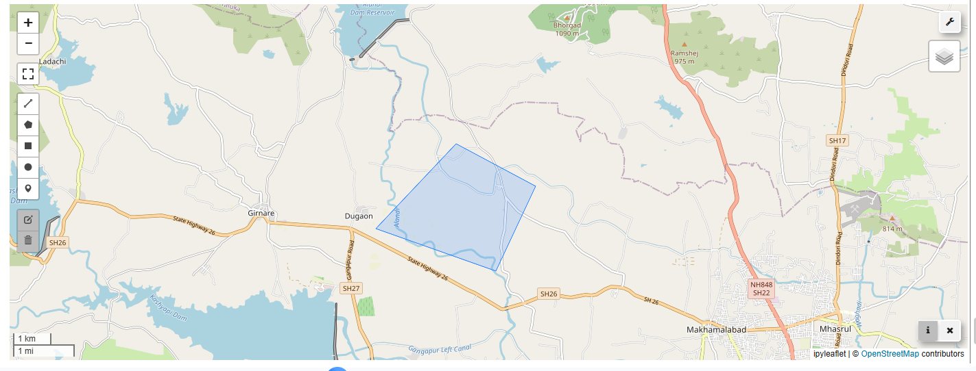
Advanced Interactive Features¶
from ipyleaflet import DrawControl
from ipywidgets import Output

# Create map with drawing capabilities
m = Map(center=nashik_center, zoom=10)

# Create output widget for displaying drawn features
output = Output()

# Create draw control
draw_control = DrawControl(
    polygon={'shapeOptions': {'color': '#6bc2e5', 'weight': 4, 'opacity': 1.0}},
    polyline={'shapeOptions': {'color': '#6bc2e5', 'weight': 4, 'opacity': 1.0}},
    circle={'shapeOptions': {'fillColor': '#efed69', 'color': 'black', 'fillOpacity': 1.0}},
    rectangle={'shapeOptions': {'fillColor': '#fca45d', 'color': 'black', 'fillOpacity': 1.0}},
)

# Handle draw events
def handle_draw(target, action, geo_json):
    with output:
        print(f"Action: {action}")
        print(f"GeoJSON: {geo_json}")
        if action == 'created':
            print(f"New {geo_json['geometry']['type']} created")
        elif action == 'deleted':
            print("Feature deleted")
        print("-" * 50)

draw_control.on_draw(handle_draw)
m.add_control(draw_control)

# Display map with output
VBox([m, output])
Problem 1: Regional Analysis Map¶
Create a comprehensive map of a specific region:
# TODO:
# 1. Filter data for a specific continent
# 2. Create a matplotlib subplot with 2 maps
# 3. Show population and GDP in different maps
# 4. Add appropriate legends and titles
# 5. Style the maps professionally

# Your code here
Problem 2: Interactive City Explorer¶
Build an interactive map for exploring cities:
# TODO:
# 1. Create a leafmap with satellite basemap
# 2. Add countries with population styling
# 3. Add cities with size based on population
# 4. Create informative popups for cities
# 5. Add layer controls and measurement tools

# Your code here
Problem 3: Comparison Map¶
Create a split-screen comparison:
# TODO:
# 1. Create a leafmap with split view
# 2. Show different data on each side
# 3. Add appropriate styling
# 4. Include popups and controls
# 5. Export as HTML

# Your code here
Key Takeaways¶
What You've Learned
- Static Visualization: Creating publication-quality maps with matplotlib
- Interactive Mapping: Building engaging maps with leafmap
- Layer Management: Adding and styling multiple data layers
- User Interaction: Implementing popups and controls
- Export Options: Saving maps for sharing and printing
Best Practices
- Choose appropriate basemaps for your data
- Use consistent styling across layers
- Provide informative popups and legends
- Test interactivity before sharing
- Consider your audience when designing maps
- Always include proper attribution