Module 4: Raster Data & Analysis¶
Learning Goals¶
- Explain raster data in simple terms (grid of pixels, cell values, resolution, extent, CRS, NoData)
- Load and inspect raster files with rasterio
- Perform raster calculations and statistics
- Clip rasters using vector boundaries
- Combine raster and vector data analysis
- Handle NoData values and data types
- Complete the basics assignment (bundled
Tiff_1.tif/Tiff_2.tif, smallrasterioscripts) before the Advance Analytics walkthrough
Introduction to Raster Data¶
In the simplest terms, a raster is a checkerboard of numbers on a map. Imagine graph paper laid over an area: every square (cell) holds one value—elevation, temperature, a land-cover code, or how “bright” the ground is in a satellite band. The squares are usually the same size on the ground (for example 30 m × 30 m), and together they cover a rectangle of territory. There is no outline of a road or a lake stored as a line or polygon; instead, each square stores whatever is true in that patch of ground (often an average or sample for the whole square).
It helps to think of a raster as a 2D table (rows × columns) where each cell has (row, column) → value, plus metadata that says where that table sits on Earth (origin, cell size, CRS). A photo is also a raster: each pixel has red, green, blue values. GIS rasters use the same grid idea, but the “colour” might be height, rainfall, or forest = 5, water = 1 instead of RGB.
Key ideas (plain language)¶
- Grid — Fixed rows and columns of cells (often called pixels). Each cell is one ground patch.
- Cell value — Usually one number per cell; satellite scenes can have several numbers per cell (bands), like extra columns glued to the same square.
- Resolution — How wide one cell is on the ground (e.g. 10 m). Smaller cells = more detail = more rows and columns and bigger files.
- Extent — The outer box of the raster: smallest and largest x / y (or lon / lat) the grid covers.
- CRS — The rule that turns column/row positions into real places on Earth (see Module 2 if CRS is new to you).
- NoData — A sentinel value meaning “no measurement here” (cloud, sea mask, edge of study area). It is not the same as zero.
graph TD
    A[Raster Data] --> B[Grid Structure]
    A --> C[Cell Values]
    A --> D[Spatial Reference]
    B --> E[Rows & Columns]
    B --> F[Resolution]
    C --> G[Continuous Values]
    C --> H[Categorical Values]
    D --> I[Coordinate System]
    D --> J[Extent/Bounds]
Common Raster Data Types¶
Digital Elevation Models (DEMs): Store terrain height values, essential for topographic analysis, watershed modeling, and visibility studies.
Satellite Imagery: Multispectral data capturing different wavelengths of light. Each band represents different portions of the electromagnetic spectrum:
- Visible bands (Red, Green, Blue): What human eyes can see
- Near-Infrared (NIR): Useful for vegetation analysis
- Thermal bands: Measure surface temperature
- Radar bands: Can penetrate clouds and work day/night
Climate Data: Temperature, precipitation, humidity measurements over time and space.
Population Density: Number of people per unit area, often derived from census data.
Land Cover/Land Use: Classification of Earth's surface (forest, urban, water, agriculture).
Raster vs Vector Data¶
| Aspect | Raster | Vector |
|---|---|---|
| Structure | Grid of cells | Points, lines, polygons |
| Best for | Continuous phenomena | Discrete objects |
| Storage | Fixed grid size | Variable based on complexity |
| Analysis | Mathematical operations | Geometric operations |
| Examples | Temperature, elevation | Roads, boundaries, buildings |
Understanding Raster Resolution¶
Spatial Resolution: The ground distance represented by each pixel
- High resolution (1-5m): Detailed analysis, small areas
- Medium resolution (10-30m): Regional studies, land cover mapping
- Low resolution (100m-1km): Global studies, climate modeling
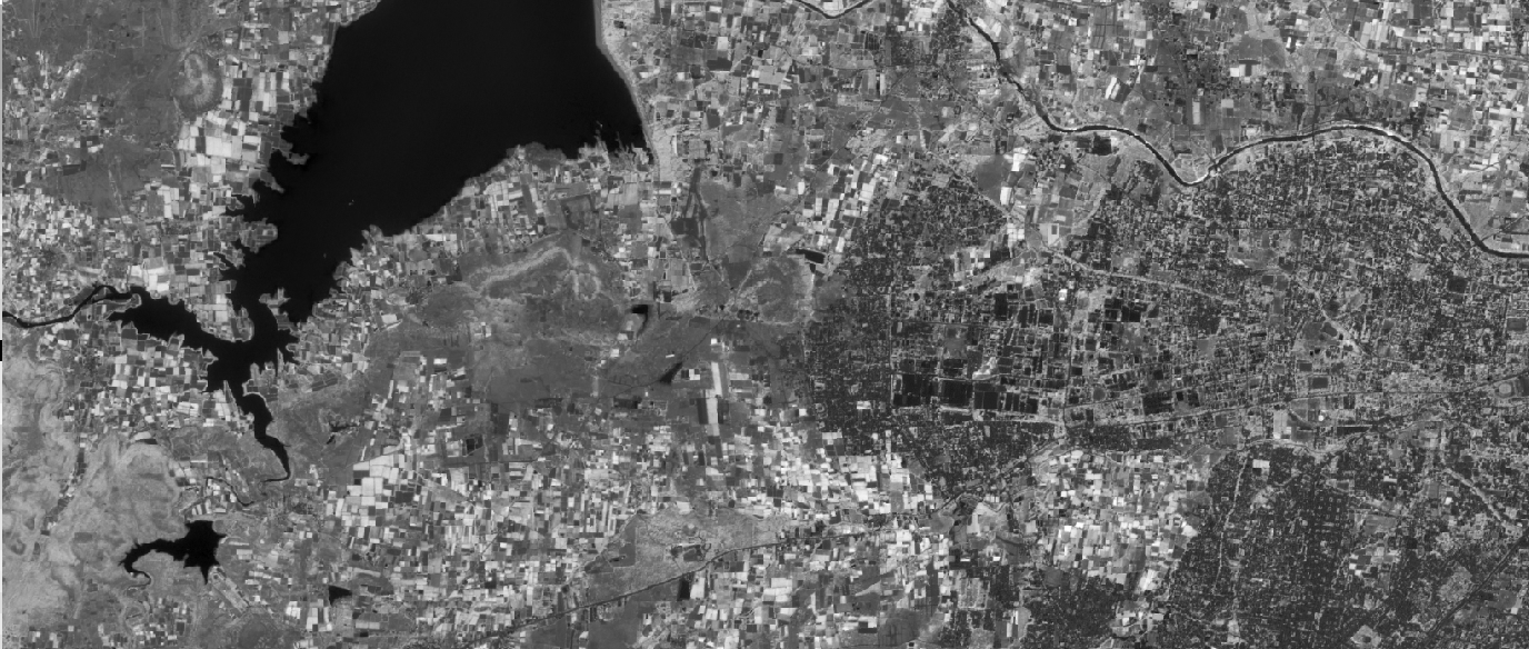
Same scene in GeoTIFF: 10 m vs 250 m spatial resolution¶
Spatial resolution is the ground width of one pixel. A 10 m GeoTIFF divides the landscape into small squares; a 250 m GeoTIFF uses much larger squares to cover the same hills, fields, and settlements. Both can be valid products—they answer different questions.
| 10 m pixels | 250 m pixels | |
|---|---|---|
| Detail | Sharper: narrow roads, field edges, and small patches stay visible at map scale | Smoother / blockier: one value averages a big patch of ground, so fine features blend together |
| Rows & columns | Many cells for the same map extent → larger file, slower to process | Few cells → smaller file, faster summaries over big regions |
| Typical use | Site-scale work, building footprints, trail mapping | Regional or global overview, climate grids, coarse land cover |
Important: lower resolution (bigger metres per pixel) does not mean a “clearer” picture in the sense of sharp edges—it usually means less spatial detail, but the map can look less noisy when you are zoomed out, because each pixel hides small variations inside its big footprint. Higher resolution (smaller metres per pixel) is what makes small features easier to see when you zoom in.
Below, the same kind of GeoTIFF is shown at ~10 m and ~250 m cell size (illustrative exports). Compare how edges and texture change.
Temporal Resolution: How often data is collected
- Daily: Weather data, some satellites
- Weekly/Monthly: Vegetation monitoring
- Annual: Land cover change detection
Spectral Resolution: Number and width of spectral bands
- Panchromatic: Single band (black and white)
- Multispectral: 3-10 bands (RGB + infrared)
- Hyperspectral: 100+ narrow bands
Raster File Formats¶
GeoTIFF (.tif/.tiff): Most common format, supports georeferencing and multiple bands
Sample GeoTIFFs for practice (in assets/tiff/ in this repo):
Click to download Tiff_1.tif Click to download Tiff_2.tif
Preview a GeoTIFF in the browser
If you want a quick visual check that a file opens on a map with plausible alignment—without QGIS or Python yet—try the free Pozyx Online GeoTIFF Viewer (upload your .tif in the browser). It is aimed at RGB-style rasters, common CRS tags, and fast validation; for many-band scientific rasters, COG streaming, or heavy analysis, use QGIS / rasterio as described later in this module. See Pozyx’s page for current limits and what the tool does not support.
NetCDF (.nc): Excellent for scientific data with multiple dimensions (time, depth)
HDF (.hdf): Hierarchical format for complex scientific datasets
JPEG2000 (.jp2): Compressed format with good quality retention
ESRI Grid: Proprietary format used by ArcGIS
Raster Coordinate Systems¶
Geographic Coordinates: Latitude/longitude in degrees - Good for: Global datasets, web mapping - Units: Decimal degrees - Example: WGS84 (EPSG:4326)
Projected Coordinates: Flat map projections in linear units - Good for: Area calculations, distance measurements - Units: Meters, feet - Example: UTM zones, State Plane
Raster Data Quality Considerations¶
Accuracy: How close values are to true measurements
Precision: Consistency of repeated measurements
Completeness: Percentage of area covered (vs NoData)
Currency: How recent the data is
Lineage: Documentation of data sources and processing steps
Raster bands and spectral indices¶
What are raster bands?¶
A raster band is one layer of values inside a raster dataset.
A raster image may contain one band or multiple bands.
Each band stores a specific measurement for every pixel.
Examples:
- visible light
- near infrared
- shortwave infrared
- elevation
- temperature
You can think of bands like stacked layers.
Each layer has:
- same width
- same height
- different values
Example:
A satellite image may store:
- Band 1 → Blue
- Band 2 → Green
- Band 3 → Red
- Band 4 → Near Infrared
The same pixel location will have one value in each band.
Example:
| Pixel location | Blue | Green | Red | NIR |
|---|---|---|---|---|
| Row 1, Col 1 | 34 | 45 | 55 | 120 |
| Row 1, Col 2 | 30 | 40 | 50 | 115 |
| Row 2, Col 1 | 32 | 44 | 54 | 118 |
This allows comparison between wavelengths.
Common raster bands¶
Different satellites may use different band numbers.
Example:
| Band | Name | Common use |
|---|---|---|
| 1 | Blue | water, coastline |
| 2 | Green | vegetation |
| 3 | Red | plant health |
| 4 | Near Infrared (NIR) | vegetation analysis |
| 5 | SWIR 1 | moisture |
| 6 | SWIR 2 | soil and geology |
| 7 | Thermal | heat |
Why bands matter¶
Different land surfaces reflect light differently.
Example:
| Surface | Blue | Red | NIR |
|---|---|---|---|
| Water | low | low | very low |
| Soil | medium | medium | medium |
| Healthy vegetation | medium | low | high |
| Built-up | medium | medium | medium-high |
Because of this, we can combine bands mathematically and create spectral indices.
What are spectral indices?¶
A spectral index is a formula created using raster bands.
It highlights a specific land condition such as:
- vegetation
- water
- soil
- burned areas
- urban areas
Indices are calculated pixel by pixel.
Result:
- one new raster
- each pixel stores calculated value
NDVI — Normalized Difference Vegetation Index¶
NDVI measures vegetation health.
Healthy vegetation reflects:
- high NIR
- low Red
Formula:
NDVI = (NIR - Red) / (NIR + Red)
````

Example:

| Red | NIR |  NDVI |
| --: | --: | ----: |
|  40 | 140 |  0.56 |
|  70 |  75 |  0.03 |
|  80 |  50 | -0.23 |

Typical NDVI values:

|      NDVI | Meaning                  |
| --------: | ------------------------ |
|       < 0 | water / clouds           |
|   0 – 0.2 | bare soil                |
| 0.2 – 0.5 | vegetation               |
|     > 0.5 | dense healthy vegetation |

Uses:

* crop monitoring
* forest analysis
* drought detection

---

## EVI — Enhanced Vegetation Index

EVI improves vegetation detection where NDVI may saturate.

It uses:

* NIR
* Red
* Blue

Formula:

```text
EVI = 2.5 × (NIR - Red) / (NIR + 6×Red - 7.5×Blue + 1)
Example:
| Blue | Red | NIR | EVI |
|---|---|---|---|
| 20 | 40 | 140 | 0.63 |
| 25 | 60 | 100 | 0.31 |
Uses:
- dense vegetation
- tropical forests
- crop monitoring
NDWI — Normalized Difference Water Index¶
NDWI highlights water.
Uses:
- Green
- NIR
Formula:
Example:
| Green | NIR | NDWI |
|---|---|---|
| 80 | 20 | 0.60 |
| 40 | 90 | -0.38 |
Uses:
- lakes
- rivers
- water bodies
NDBI — Normalized Difference Built-up Index¶
Detects urban and built-up areas.
Uses:
- SWIR
- NIR
Formula:
Example:
| SWIR | NIR | NDBI |
|---|---|---|
| 130 | 80 | 0.24 |
| 70 | 120 | -0.26 |
Uses:
- urban growth
- buildings
- roads
SAVI — Soil Adjusted Vegetation Index¶
Improves vegetation detection where soil is visible.
Formula:
Usually:
Uses:
- agriculture
- dry areas
- sparse vegetation
BSI — Bare Soil Index¶
Highlights exposed soil.
Formula:
Uses:
- barren land
- soil analysis
Summary¶
Raster bands store values in separate image layers.
By combining bands using formulas we can create indices.
Common indices:
| Index | Uses |
|---|---|
| NDVI | vegetation |
| EVI | dense vegetation |
| NDWI | water |
| NDBI | built-up |
| SAVI | soil + vegetation |
| BSI | bare soil |
These indices are widely used in:
- agriculture
- remote sensing
- environmental monitoring
- land use mapping
- GIS analysis
Download satellite data (Sentinel-2)¶
In this section we will learn how to download satellite imagery from Sentinel-2 using Python and cloud-based geospatial catalogs.
Sentinel-2 is a satellite mission from the European Space Agency (ESA).
It captures Earth observation imagery useful for:
- vegetation monitoring
- agriculture
- land use mapping
- flood analysis
- forest monitoring
- water resources
- urban growth
Sentinel-2 imagery is freely available and commonly used in GIS and remote sensing.
It provides:
- 10 m resolution → Blue, Green, Red, NIR
- 20 m resolution → Red Edge, SWIR
- 60 m resolution → atmospheric bands
Common useful bands:
| Band | Name | Resolution |
|---|---|---|
| B2 | Blue | 10 m |
| B3 | Green | 10 m |
| B4 | Red | 10 m |
| B8 | Near Infrared | 10 m |
| B11 | SWIR | 20 m |
| B12 | SWIR | 20 m |
Sentinel-2 data can be downloaded from several cloud catalogs.
A common workflow:
- search imagery by location
- filter by date
- filter by cloud cover
- select required bands
- load imagery into Python
- process raster
1. Microsoft Planetary Computer¶
Microsoft Planetary Computer is a cloud platform that provides access to large public geospatial datasets.
It includes:
- Sentinel-2
- Landsat
- DEM datasets
- climate data
- land cover
Website:
https://planetarycomputer.microsoft.com/
It uses the STAC (SpatioTemporal Asset Catalog) standard.
This means we can search data using:
- bounding box
- geometry
- date range
- cloud cover
- collection name
Example collections:
sentinel-2-l2alandsat-c2-l2
Benefits:
- free access
- cloud hosted
- fast search
- no manual downloading needed
- ready for Python workflows
Typical workflow:
- open catalog
- search Sentinel-2
- choose date + area
- filter by cloud cover
- access raster assets
Useful for:
- satellite analysis
- time series
- NDVI
- agriculture monitoring
2. PySTAC¶
PySTAC is a Python library for working with STAC catalogs.
STAC is a standard format used to describe geospatial datasets.
PySTAC helps read:
- catalogs
- collections
- items
- raster assets
It lets us:
- open STAC catalog
- search datasets
- inspect metadata
- list available bands
- access image links
Example metadata available:
- acquisition date
- cloud cover
- satellite name
- band URLs
- projection
Useful for:
- discovering satellite scenes
- reading metadata
- selecting imagery
Simple idea:
- Planetary Computer stores the data
- PySTAC reads the catalog and metadata
Typical workflow:
- connect to catalog
- search Sentinel-2
- read returned items
- inspect bands
- select image
Useful when:
- browsing scenes
- checking metadata
- building automated search
3. ODC-STAC¶
ODC-STAC stands for:
Open Data Cube + STAC
It is a Python library used to load STAC items directly into analysis-ready arrays.
While PySTAC helps discover data, ODC-STAC helps load it for analysis.
It works well with:
- xarray
- NumPy
- Rasterio
It helps us:
- load selected bands
- clip to area
- combine scenes
- stack rasters
- prepare analysis-ready data
Example uses:
- NDVI calculation
- cloud filtering
- time-series analysis
- mosaics
Typical workflow:
- search Sentinel-2 using STAC
- select items
- load bands with ODC-STAC
- calculate indices
- export results
Benefits:
- fast loading
- multiple scenes
- direct analysis
- works well with raster workflows
Quick comparison¶
| Tool | Main use |
|---|---|
| Microsoft Planetary Computer | cloud catalog + satellite storage |
| PySTAC | search and read STAC metadata |
| ODC-STAC | load imagery for analysis |
Simple workflow:
Microsoft Planetary Computer
        ↓
Search Sentinel-2 scenes
        ↓
PySTAC reads catalog + metadata
        ↓
ODC-STAC loads imagery
        ↓
Raster analysis with Python
Search available Sentinel-2 data¶
Before downloading satellite imagery, we usually search available scenes for our study area.
This helps us:
- check whether imagery exists
- filter by date
- filter by cloud cover
- inspect available scenes
- choose the best image before loading bands
For Sentinel-2, a common workflow is:
- define study area (GeoJSON)
- choose start and end date
- choose maximum cloud cover
- search catalog
- inspect results
- select image
We can search data directly from Microsoft Planetary Computer using PySTAC Client.
Install required libraries¶
Libraries used:
- pystac-client → search STAC catalog
- planetary-computer → Microsoft Planetary Computer access
- odc-stac → load imagery
- geopandas → vector boundaries
- pandas → tabular results
Search available Sentinel-2 imagery¶
This program:
- connects to Microsoft Planetary Computer
- searches Sentinel-2 Level-2A
- filters by:
- polygon boundary
- date range
- cloud cover
- returns results as JSON
"""
Search Sentinel-2 imagery from Planetary Computer
and return JSON.
"""

import json
from pystac_client import Client

STAC_URL = "https://planetarycomputer.microsoft.com/api/stac/v1"


def search_sentinel2(
    geojson_fc: dict,
    start_date: str,
    end_date: str,
    max_cloud_cover: int = 20,
):
    # --------------------------------
    # convert FeatureCollection → geometry
    # --------------------------------
    if geojson_fc["type"] == "FeatureCollection":
        geometry = geojson_fc["features"][0]["geometry"]

    elif geojson_fc["type"] == "Feature":
        geometry = geojson_fc["geometry"]

    else:
        geometry = geojson_fc

    # --------------------------------
    # connect stac
    # --------------------------------
    catalog = Client.open(STAC_URL)

    search = catalog.search(
        collections=["sentinel-2-l2a"],
        intersects=geometry,
        datetime=f"{start_date}/{end_date}",
        query={
            "eo:cloud_cover": {
                "lte": max_cloud_cover
            }
        },
    )

    items = list(search.items())

    # --------------------------------
    # no results
    # --------------------------------
    if not items:
        return {
            "count": 0,
            "results": []
        }

    # --------------------------------
    # results
    # --------------------------------
    results = []

    for item in items:
        results.append(
            {
                "id": item.id,
                "date": item.datetime.date().isoformat(),
                "datetime": item.datetime.isoformat(),
                "cloud_cover": item.properties.get(
                    "eo:cloud_cover"
                ),
                "product": item.properties.get(
                    "s2:product_uri"
                ),
                "platform": item.properties.get(
                    "platform"
                ),
            }
        )

    # sort by date
    results = sorted(
        results,
        key=lambda x: x["date"]
    )

    return {
        "count": len(results),
        "results": results,
    }


# --------------------------------
# Example
# --------------------------------

geojson_fc = {
    "type": "FeatureCollection",
    "features": [
        {
            "type": "Feature",
            "properties": {},
            "geometry": {
                "type": "Polygon",
                "coordinates": [[
                    [76.8149, 17.6984],
                    [76.8131, 17.6972],
                    [76.8155, 17.6961],
                    [76.8172, 17.6976],
                    [76.8149, 17.6984],
                ]],
            },
        }
    ],
}

data = search_sentinel2(
    geojson_fc=geojson_fc,
    start_date="2025-12-01",
    end_date="2025-12-31",
    max_cloud_cover=15,
)

print(json.dumps(data, indent=2))
Example output¶
{
  "count": 2,
  "results": [
    {
      "id": "S2A_MSIL2A_20251212T052201",
      "date": "2025-12-12",
      "datetime": "2025-12-12T05:22:01+00:00",
      "cloud_cover": 8.2,
      "product": "S2A_MSIL2A_20251212T052201",
      "platform": "sentinel-2a"
    },
    {
      "id": "S2B_MSIL2A_20251222T052201",
      "date": "2025-12-22",
      "datetime": "2025-12-22T05:22:01+00:00",
      "cloud_cover": 12.6,
      "product": "S2B_MSIL2A_20251222T052201",
      "platform": "sentinel-2b"
    }
  ]
}
Result fields¶
| Field | Meaning |
|---|---|
id |
Sentinel scene id |
date |
image date |
datetime |
exact capture time |
cloud_cover |
cloud percentage |
product |
product name |
platform |
Sentinel satellite |
Summary¶
Searching Sentinel-2 before downloading helps us:
- find available imagery
- filter low-cloud scenes
- compare dates
- select the best image
Typical workflow:
GeoJSON study area
        ↓
Search Sentinel-2
        ↓
Check cloud cover
        ↓
Choose best scene
        ↓
Load raster bands
        ↓
Calculate NDVI / analysis
Download clipped raw Sentinel-2 bands¶
Sometimes we need the original satellite bands instead of calculated indices.
Raw bands are useful for:
- NDVI / EVI calculation
- RGB image creation
- false color composites
- land cover analysis
- water detection
- remote sensing workflows
In this example we will:
- use a GeoJSON polygon
- select one Sentinel-2 scene
- load required bands
- clip exactly to polygon
- save each band as a separate GeoTIFF
This gives us raw clipped raster bands ready for GIS analysis.
Install required libraries¶
Libraries used:
- pystac-client → search STAC catalog
- planetary-computer → sign URLs
- odc-stac → load raster bands
- rasterio → raster processing
- rioxarray → clip + export
Download clipped raw bands¶
This function:
- accepts GeoJSON polygon
- accepts Sentinel-2 item id
- accepts list of bands
- clips raster
- saves TIFF files
import os
import rasterio
from shapely.geometry import shape
from pystac_client import Client
import planetary_computer as pc
from odc.stac import load
import rioxarray


STAC_URL = "https://planetarycomputer.microsoft.com/api/stac/v1"


def download_clipped_raw_bands(
    geojson_data: dict,
    item_id: str,
    bands: list,
    output_dir: str,
):
    """
    Download clipped raw Sentinel-2 bands.

    Parameters
    ----------
    geojson_data : dict
        GeoJSON Polygon / Feature / FeatureCollection

    item_id : str
        Sentinel-2 item id

    bands : list
        Example:
        ["B02", "B03", "B04", "B08"]

    output_dir : str
        Folder to save TIFFs
    """

    # --------------------------
    # geometry
    # --------------------------
    if geojson_data["type"] == "FeatureCollection":
        geom_geojson = geojson_data["features"][0]["geometry"]

    elif geojson_data["type"] == "Feature":
        geom_geojson = geojson_data["geometry"]

    else:
        geom_geojson = geojson_data

    geom = shape(geom_geojson)

    # --------------------------
    # stac
    # --------------------------
    client = Client.open(
        STAC_URL,
        modifier=pc.sign_inplace,
    )

    search = client.search(
        collections=["sentinel-2-l2a"],
        ids=[item_id],
    )

    items = list(search.items())

    if not items:
        raise ValueError(
            f"No item found for {item_id}"
        )

    signed_items = [
        pc.sign(item)
        for item in items
    ]

    # --------------------------
    # load only required bands
    # --------------------------
    ds = load(
        items=signed_items,
        geopolygon=geom,
        groupby="solar_day",
        bands=bands,
    )

    # exact polygon clip
    ds = ds.rio.clip(
        [geom],
        crs="EPSG:4326",
    )

    # first image only
    ds = ds.isel(time=0)

    # create folder
    os.makedirs(
        output_dir,
        exist_ok=True,
    )

    saved_files = []

    # --------------------------
    # save each band
    # --------------------------
    for band in bands:

        output_path = os.path.join(
            output_dir,
            f"{band}.tif",
        )

        ds[band].rio.to_raster(
            output_path
        )

        saved_files.append(
            output_path
        )

    return {
        "status": "success",
        "item_id": item_id,
        "bands": bands,
        "files": saved_files,
    }


# -----------------------------------
# Example
# -----------------------------------

res = download_clipped_raw_bands(
    geojson_data=geojson_fc,
    item_id="S2C_MSIL2A_20251214T053241_R105_T43QDF_20251214T090710",
    bands=[
        "B02",
        "B03",
        "B04",
        "B08",
    ],
    output_dir="/content/raw_bands",
)

print(res)
Example output¶
{
    "status": "success",
    "item_id": "S2C_MSIL2A_20251214T053241_R105_T43QDF_20251214T090710",
    "bands": [
        "B02",
        "B03",
        "B04",
        "B08"
    ],
    "files": [
        "/content/raw_bands/B02.tif",
        "/content/raw_bands/B03.tif",
        "/content/raw_bands/B04.tif",
        "/content/raw_bands/B08.tif"
    ]
}
Common Sentinel-2 bands¶
| Band | Name | Resolution | Use |
|---|---|---|---|
| B02 | Blue | 10 m | water / coast |
| B03 | Green | 10 m | vegetation |
| B04 | Red | 10 m | NDVI |
| B08 | NIR | 10 m | vegetation |
| B11 | SWIR | 20 m | moisture |
| B12 | SWIR | 20 m | soil |
Example band combinations¶
RGB true color:
False color vegetation:
NDVI:
EVI:
Parameters¶
| Parameter | Meaning |
|---|---|
geojson_data |
study area polygon |
item_id |
Sentinel scene id |
bands |
list of bands |
output_dir |
folder to save TIFFs |
Workflow summary¶
GeoJSON study area
        ↓
Search Sentinel-2
        ↓
Choose item_id
        ↓
Select bands
        ↓
Load raster
        ↓
Clip polygon
        ↓
Save each TIFF
Result¶
Output files can be used in:
- QGIS
- Rasterio
- NumPy
- NDVI calculation
- RGB rendering
- remote sensing analysis
Download NDVI or EVI GeoTIFF from Sentinel-2¶
After searching available Sentinel-2 scenes, the next step is to download raster bands and calculate vegetation indices.
In this example we:
- use a GeoJSON polygon as study area
- select one Sentinel-2 scene using
item_id - load required bands
- calculate:
- NDVI
- or EVI
- clip result exactly to polygon
- save output as GeoTIFF
This workflow is useful for:
- crop monitoring
- vegetation health
- remote sensing analysis
- agricultural GIS workflows
Install required libraries¶
Libraries used:
- pystac-client → search STAC catalog
- planetary-computer → sign asset URLs
- odc-stac → load raster bands
- rasterio → raster handling
- rioxarray → clipping + export
Download clipped NDVI or EVI¶
This function:
- accepts GeoJSON
- accepts Sentinel-2 item id
- calculates NDVI or EVI
- clips raster
- saves GeoTIFF
import numpy as np
import rasterio
from shapely.geometry import shape
from pystac_client import Client
import planetary_computer as pc
from odc.stac import load
import rioxarray


STAC_URL = "https://planetarycomputer.microsoft.com/api/stac/v1"


def download_clipped_index_tiff(
    geojson_data: dict,
    item_id: str,
    index: str,
    output_path: str,
):
    """
    Download clipped Sentinel-2 NDVI/EVI GeoTIFF.

    Parameters
    ----------
    geojson_data : dict
    item_id : str
    index : str ("ndvi" or "evi")
    output_path : str
    """

    # ---------------------------------
    # geometry
    # ---------------------------------
    if geojson_data["type"] == "FeatureCollection":
        geom_geojson = geojson_data["features"][0]["geometry"]
    elif geojson_data["type"] == "Feature":
        geom_geojson = geojson_data["geometry"]
    else:
        geom_geojson = geojson_data

    geom = shape(geom_geojson)

    # ---------------------------------
    # stac search by id
    # ---------------------------------
    client = Client.open(
        STAC_URL,
        modifier=pc.sign_inplace,
    )

    search = client.search(
        collections=["sentinel-2-l2a"],
        ids=[item_id],
    )

    items = list(search.items())

    if not items:
        raise ValueError(
            f"No item found for {item_id}"
        )

    signed_items = [
        pc.sign(item)
        for item in items
    ]

    # ---------------------------------
    # required bands
    # ---------------------------------
    bands = ["B04", "B08"]

    if index.lower() == "evi":
        bands.append("B02")

    # ---------------------------------
    # load clipped to polygon
    # ---------------------------------
    ds = load(
        items=signed_items,
        geopolygon=geom,
        groupby="solar_day",
        bands=bands,
    )

    # exact polygon clip
    ds = ds.rio.clip(
        [geom],
        crs="EPSG:4326",
    )

    # ---------------------------------
    # calculate index
    # ---------------------------------
    red = ds["B04"]
    nir = ds["B08"]

    if index.lower() == "ndvi":
        result = (
            (nir - red)
            / (nir + red + 1e-6)
        )

    elif index.lower() == "evi":
        blue = ds["B02"]

        result = (
            2.5
            * (nir - red)
            / (
                nir
                + 6 * red
                - 7.5 * blue
                + 1
            )
        )

    else:
        raise ValueError(
            "Supported: ndvi or evi"
        )

    # first image only
    result = result.isel(time=0)

    # ---------------------------------
    # save
    # ---------------------------------
    result.rio.to_raster(output_path)

    return {
        "status": "success",
        "item_id": item_id,
        "index": index,
        "output": output_path,
    }


# -------------------------------------
# Example
# -------------------------------------

res = download_clipped_index_tiff(
    geojson_data=geojson_fc,
    item_id="S2C_MSIL2A_20251204T053221_R105_T43QDF_20251204T091915",
    index="ndvi",
    output_path="/content/ndvi_clip.tif",
)

print(res)
Example output¶
{
    "status": "success",
    "item_id": "S2C_MSIL2A_20251204T053221_R105_T43QDF_20251204T091915",
    "index": "ndvi",
    "output": "/content/ndvi_clip.tif"
}
Supported indices¶
| Index | Bands used | Formula |
|---|---|---|
| NDVI | NIR + Red | (NIR - Red) / (NIR + Red) |
| EVI | NIR + Red + Blue | 2.5 × (NIR - Red) / (NIR + 6×Red - 7.5×Blue + 1) |
Sentinel-2 bands used¶
| Band | Name | Resolution |
|---|---|---|
| B02 | Blue | 10 m |
| B04 | Red | 10 m |
| B08 | Near Infrared | 10 m |
Parameters¶
| Parameter | Meaning |
|---|---|
geojson_data |
study area polygon |
item_id |
Sentinel-2 scene id |
index |
"ndvi" or "evi" |
output_path |
output GeoTIFF location |
Workflow summary¶
GeoJSON study area
        ↓
Search Sentinel-2
        ↓
Choose item_id
        ↓
Load bands
        ↓
Calculate NDVI / EVI
        ↓
Clip to polygon
        ↓
Save GeoTIFF
Result¶
The output file is a clipped raster GeoTIFF.
It can be used in:
- QGIS
- Rasterio
- GeoPandas workflows
- agricultural analysis
- vegetation monitoring
Download LULC GeoTIFF from Sentinel-2¶
Along with downloading raster bands and vegetation indices, we can also create a simple Land Use / Land Cover (LULC) raster.
LULC helps classify land into categories such as:
- water
- built-up area
- barren/open soil
- sparse vegetation
- dense vegetation
In this example we:
- use a GeoJSON polygon
- search Sentinel-2 scenes
- filter by date and cloud cover
- create a cloud-free composite
- calculate indices
- classify land cover
- clip exactly to polygon
- save output as GeoTIFF
This workflow is useful for:
- land use mapping
- agriculture monitoring
- vegetation analysis
- urban growth
- GIS raster classification
Install required libraries¶
Libraries used:
- pystac-client → search STAC
- planetary-computer → sign imagery
- odc-stac → load raster bands
- geopandas → polygon handling
- rasterio → save raster
- rioxarray → clipping
- scipy → smoothing filter
Download LULC raster¶
This function:
- searches Sentinel-2
- removes clouds
- creates median composite
- calculates:
- NDVI
- NDBI
- MNDWI
- classifies pixels
- saves LULC GeoTIFF
import numpy as np
import rasterio
import geopandas as gpd
from shapely.geometry import shape
from rasterio.mask import mask as rio_mask
from pystac_client import Client
import planetary_computer as pc
from odc.stac import load
from scipy.ndimage import median_filter


STAC_URL = "https://planetarycomputer.microsoft.com/api/stac/v1"


def download_lulc_tiff(
    geojson_data: dict,
    date_range: str,
    cloud_cover: int,
    output_path: str,
    max_items: int = 10,
    resolution: int = 20,
):
    """
    Download clipped Sentinel-2 LULC GeoTIFF.

    Classes
    -------
    0 -> Water
    1 -> Built-up
    2 -> Barren/Open soil
    3 -> Sparse vegetation
    4 -> Dense vegetation
    255 -> NoData
    """

    # --------------------------------
    # geometry
    # --------------------------------
    if geojson_data["type"] == "FeatureCollection":
        geom_geojson = geojson_data["features"][0]["geometry"]

    elif geojson_data["type"] == "Feature":
        geom_geojson = geojson_data["geometry"]

    else:
        geom_geojson = geojson_data

    geom = shape(geom_geojson)

    gdf = gpd.GeoDataFrame(
        geometry=[geom],
        crs="EPSG:4326",
    )

    bbox = tuple(gdf.total_bounds)

    utm_crs = gdf.estimate_utm_crs()

    # --------------------------------
    # search stac
    # --------------------------------
    client = Client.open(STAC_URL)

    search = client.search(
        collections=["sentinel-2-l2a"],
        intersects=geom.__geo_interface__,
        datetime=date_range,
        query={
            "eo:cloud_cover": {
                "lt": cloud_cover
            }
        },
    )

    items = sorted(
        search.items(),
        key=lambda x: x.properties.get(
            "eo:cloud_cover",
            100,
        ),
    )[:max_items]

    if not items:
        raise ValueError(
            "No scenes found"
        )

    signed_items = [
        pc.sign(item)
        for item in items
    ]

    # --------------------------------
    # load bands
    # --------------------------------
    ds = load(
        items=signed_items,
        bands=[
            "B02",
            "B03",
            "B04",
            "B08",
            "B11",
            "SCL",
        ],
        crs=utm_crs,
        resolution=resolution,
        bbox=bbox,
        groupby="solar_day",
    )

    # --------------------------------
    # cloud mask
    # --------------------------------
    scl = ds["SCL"]

    cloud_mask = scl.isin(
        [1, 3, 8, 9, 10, 11]
    )

    blue = ds["B02"].where(
        ~cloud_mask
    ).astype("float32")

    green = ds["B03"].where(
        ~cloud_mask
    ).astype("float32")

    red = ds["B04"].where(
        ~cloud_mask
    ).astype("float32")

    nir = ds["B08"].where(
        ~cloud_mask
    ).astype("float32")

    swir = ds["B11"].where(
        ~cloud_mask
    ).astype("float32")

    # median composite
    blue = blue.median(dim="time")
    green = green.median(dim="time")
    red = red.median(dim="time")
    nir = nir.median(dim="time")
    swir = swir.median(dim="time")

    # --------------------------------
    # indices
    # --------------------------------
    def safe_index(a, b):
        denom = a + b

        return np.where(
            denom == 0,
            np.nan,
            (a - b) / denom,
        )

    b = blue.values
    g = green.values
    r = red.values
    n = nir.values
    s = swir.values

    ndvi = safe_index(n, r)

    ndbi = safe_index(s, n)

    mndwi = safe_index(g, s)

    # --------------------------------
    # classification
    # --------------------------------
    lulc = np.full(
        ndvi.shape,
        255,
        dtype=np.uint8,
    )

    valid = (
        np.isfinite(ndvi)
        & np.isfinite(ndbi)
        & np.isfinite(mndwi)
    )

    water = (
        valid
        & (mndwi > 0.1)
        & (mndwi > ndvi)
    )
    lulc[water] = 0

    dense_veg = (
        valid
        & ~water
        & (ndvi > 0.5)
    )
    lulc[dense_veg] = 4

    sparse_veg = (
        valid
        & ~water
        & ~dense_veg
        & (ndvi >= 0.2)
        & (ndvi <= 0.5)
    )
    lulc[sparse_veg] = 3

    builtup = (
        valid
        & ~water
        & ~dense_veg
        & ~sparse_veg
        & (ndbi > 0)
        & (ndvi < 0.2)
    )

    lulc[builtup] = 1

    barren = (
        valid
        & (lulc == 255)
    )

    lulc[barren] = 2

    # --------------------------------
    # smoothing
    # --------------------------------
    filtered = median_filter(
        lulc,
        size=3,
    )

    filtered[
        lulc == 255
    ] = 255

    lulc = filtered

    # --------------------------------
    # save temp
    # --------------------------------
    geobox = ds.odc.geobox

    temp_path = (
        output_path
        + ".tmp.tif"
    )

    with rasterio.open(
        temp_path,
        "w",
        driver="GTiff",
        height=lulc.shape[0],
        width=lulc.shape[1],
        count=1,
        dtype=rasterio.uint8,
        crs=geobox.crs,
        transform=geobox.transform,
        nodata=255,
    ) as dst:
        dst.write(
            lulc,
            1,
        )

    # --------------------------------
    # exact clip
    # --------------------------------
    gdf_utm = gdf.to_crs(
        utm_crs
    )

    geom_utm = (
        gdf_utm.geometry.values[0]
    )

    with rasterio.open(
        temp_path
    ) as src:

        clipped, transform = rio_mask(
            src,
            [geom_utm.__geo_interface__],
            crop=True,
            nodata=255,
        )

        meta = src.meta.copy()

    meta.update(
        {
            "height": clipped.shape[1],
            "width": clipped.shape[2],
            "transform": transform,
            "nodata": 255,
        }
    )

    with rasterio.open(
        output_path,
        "w",
        **meta,
    ) as dst:
        dst.write(
            clipped[0],
            1,
        )

    return {
        "status": "success",
        "date_range": date_range,
        "cloud_cover": cloud_cover,
        "output": output_path,
        "classes": {
            0: "Water",
            1: "Built-up",
            2: "Barren",
            3: "Sparse vegetation",
            4: "Dense vegetation",
            255: "NoData",
        },
    }
Example¶
geojson_fc = {
  "type": "FeatureCollection",
  "features": [
    {
      "type": "Feature",
      "properties": {},
      "geometry": {
        "type": "Polygon",
        "coordinates": [[
          [73.658151, 20.034861],
          [73.658151, 19.977499],
          [73.771634, 19.977499],
          [73.771634, 20.034861],
          [73.658151, 20.034861]
        ]]
      }
    }
  ]
}

res = download_lulc_tiff(
    geojson_data=geojson_fc,
    date_range="2025-01-01/2025-03-31",
    cloud_cover=20,
    output_path="/content/lulc_2025.tif",
)

print(res)
LULC classes¶
| Value | Class |
|---|---|
| 0 | Water |
| 1 | Built-up |
| 2 | Barren/Open soil |
| 3 | Sparse vegetation |
| 4 | Dense vegetation |
| 255 | NoData |
Indices used¶
| Index | Purpose |
|---|---|
| NDVI | vegetation |
| NDBI | built-up |
| MNDWI | water |
Workflow summary¶
GeoJSON polygon
        ↓
Search Sentinel-2
        ↓
Filter cloud cover
        ↓
Load bands
        ↓
Cloud mask
        ↓
Median composite
        ↓
Calculate indices
        ↓
Classify pixels
        ↓
Clip polygon
        ↓
Save GeoTIFF
Result¶
Output can be opened in:
- QGIS
- Rasterio
- GIS software
Useful for:
- land cover mapping
- agriculture
- vegetation monitoring
- urban analysis
What is Rasterio?¶
Rasterio is a Python library used to work with raster geospatial data such as satellite images, elevation maps, land cover maps, and other grid-based datasets.
Raster data stores information in the form of rows and columns of pixels, where each pixel contains a value. These values may represent things like color, height, temperature, rainfall, or vegetation.
Rasterio provides a simple Python interface to open, read, analyze, and write raster files. It is built on top of GDAL and is designed specifically for geospatial raster processing.
With Rasterio we can:
- read raster files such as GeoTIFF
- check raster metadata
- access pixel values
- crop rasters
- mask rasters using vector boundaries
- save processed raster files
Rasterio works well with:
- NumPy for raster calculations
- GeoPandas for vector data
- Shapely for geometry operations
In simple terms:
- Shapely works with geometry
- GeoPandas works with vector layers
- Rasterio works with raster grids
Rasterio is widely used in GIS and remote sensing for tasks such as:
- satellite image analysis
- digital elevation model processing
- raster clipping
- land use classification
- environmental monitoring
In short:
Rasterio is a Python GIS library used to read, analyze, and write raster geospatial data.
1. Open and read a raster file¶
import rasterio

path = "assets/tiff/Tiff_1.tif"  # bundled practice GeoTIFF
with rasterio.open(path) as src:
    band1 = src.read(1)          # 2D NumPy array, first band (height × width)
    profile = src.profile        # driver, dtype, nodata, transform, crs, size
    crs_epsg = src.crs.to_epsg() if src.crs else None
    crs_label = f"EPSG:{crs_epsg}" if crs_epsg else str(src.crs)
    print(src.shape, crs_label, src.dtypes[0])
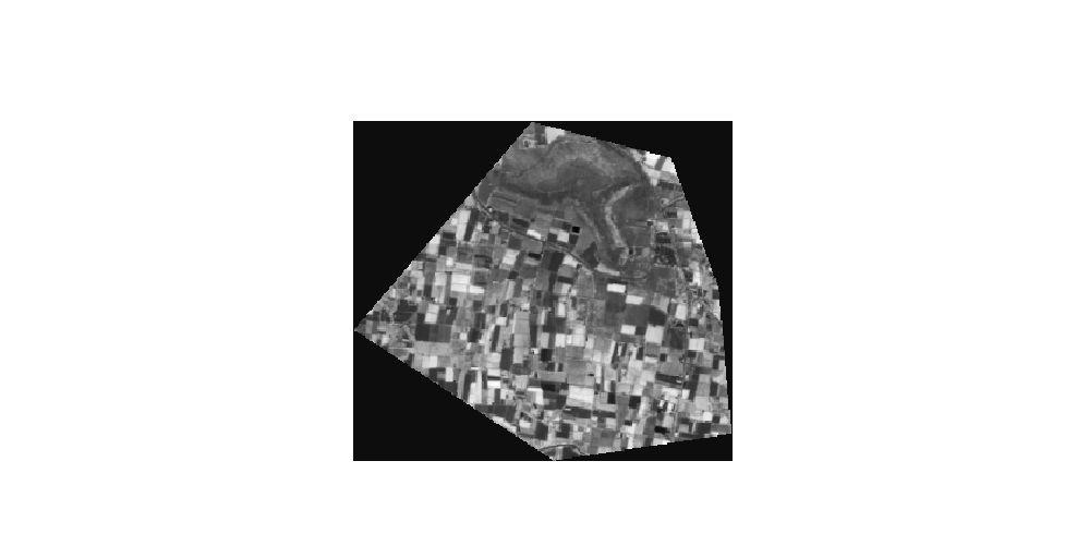
Example output for Tiff_1.tif:
read(1) loads band 1 into memory; for large files you can use windows or out_shape later to read only part of a band.
2. What are “raster statistics”?¶
Statistics here are numeric summaries of the pixel values in a band (or in a region you care about): minimum, maximum, mean (average), standard deviation, percentiles, counts of valid pixels, and so on. They answer questions like “how high is this DEM on average?” or “what range do reflectance values span?” You usually ignore NoData when computing them so missing cells do not skew the result.
3. Calculate statistics (one band, respect NoData)¶
import numpy as np
import rasterio

with rasterio.open("assets/tiff/Tiff_1.tif") as src:
    arr = src.read(1).astype("float64")
    nodata = src.nodata

    if nodata is not None:
        arr = np.where(arr == nodata, np.nan, arr)

# Basic stats
print("Min:", np.nanmin(arr))
print("Max:", np.nanmax(arr))
print("Mean:", np.nanmean(arr))
print("Median:", np.nanmedian(arr))
print("Std Dev:", np.nanstd(arr))
print("Variance:", np.nanvar(arr))

# Percentiles
print("25th Percentile:", np.nanpercentile(arr, 25))
print("50th Percentile (Median):", np.nanpercentile(arr, 50))
print("75th Percentile:", np.nanpercentile(arr, 75))

# Count info
print("Total Pixels:", arr.size)
print("Valid Pixels:", np.count_nonzero(~np.isnan(arr)))
print("NoData Pixels:", np.count_nonzero(np.isnan(arr)))
Example output when run on the bundled Tiff_1.tif:
Min: -0.11472345888614655
Max: 0.6778202652931213
Mean: 0.24052893210664816
Median: 0.22149499505758286
Std Dev: 0.13968990308740697
Variance: 0.019513269024569155
25th Percentile: 0.15612491592764854
50th Percentile (Median): 0.22149499505758286
75th Percentile: 0.32683808356523514
Total Pixels: 1150796
Valid Pixels: 1150796
NoData Pixels: 0
4. Filter pixels by value (keep cells in a range, mask the rest)¶
Build a boolean mask, then either write a new GeoTIFF or set unwanted pixels to NoData before saving.
import numpy as np
import rasterio
from rasterio.enums import Resampling
with rasterio.open("/content/Tiff_1.tif") as src:
arr = src.read(1).astype("float32")
profile = src.profile.copy()
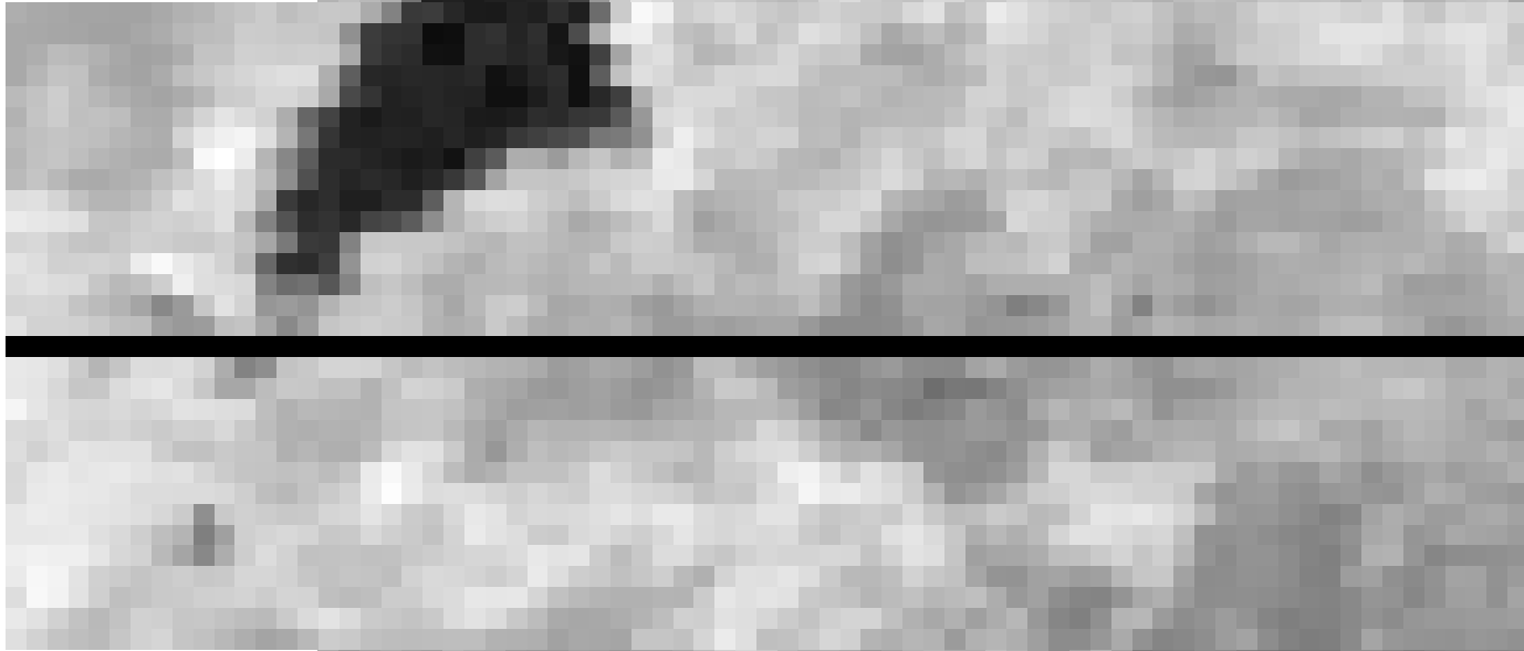
mask = (arr >= 0.1) & (arr <= 0.5) # keep elevations 100–500 (example)
out = np.where(mask, arr, src.nodata).astype(profile["dtype"])
profile.update(dtype=out.dtype, count=1, compress="deflate")
with rasterio.open("/content/Tiff_1_filter.tif", "w", **profile) as dst:
dst.write(out, 1)
Example visualization (bundled Tiff_1.tif: band 1 before masking, then after keeping only the middle value range and setting the rest to NoData—the same idea as the code above):
Adjust thresholds to your units; always set nodata in profile if you use a sentinel.
5. Clip a raster using a polygon¶
rasterio.mask.mask expects an iterable of GeoJSON-like geometries: plain Python dicts with "type" and "coordinates" (same structure as .geojson on disk). The polygon’s coordinate order must match the raster’s CRS (for example lon/lat if the DEM is EPSG:4326; if the DEM is in metres, use projected corners instead, or reproject the polygon first).
Polygon inline as GeoJSON (dict)
import rasterio
from rasterio.mask import mask

# GeoJSON Polygon: outer ring must close (first point = last point)
clip_poly = {
    "type": "Polygon",
    "coordinates": [
        [
            [
              73.71042841436719,
              20.09023103896574
            ],
            [
              73.69665791730623,
              20.074091366211377
            ],
            [
              73.71214563805651,
              20.063933096227032
            ],
            [
              73.7259168550645,
              20.066013154915694
            ],
            [
              73.72492563666324,
              20.077312229882054
            ],
            [
              73.72123577059406,
              20.087440203990184
            ],
            [
              73.71042841436719,
              20.09023103896574
            ]
        ]
    ],
}
geom = [clip_poly]

with rasterio.open("/content/Tiff_1.tif") as src:
    clipped, transform = mask(src, geom, crop=True, nodata=src.nodata)
    meta = src.meta.copy()
    meta.update({"height": clipped.shape[1], "width": clipped.shape[2], "transform": transform})

with rasterio.open("/content/Tiff_1_clipped.tif", "w", **meta) as dst:
    dst.write(clipped)
Example visualization (clipped, cropped raster after mask(..., crop=True) on Tiff_1.tif with the polygon above):
6. Merge two rasters into one mosaic¶
rasterio.merge.merge aligns inputs on a common grid and pastes them into a larger array (same CRS and compatible bands work best; otherwise reproject first).
import rasterio
from rasterio.merge import merge
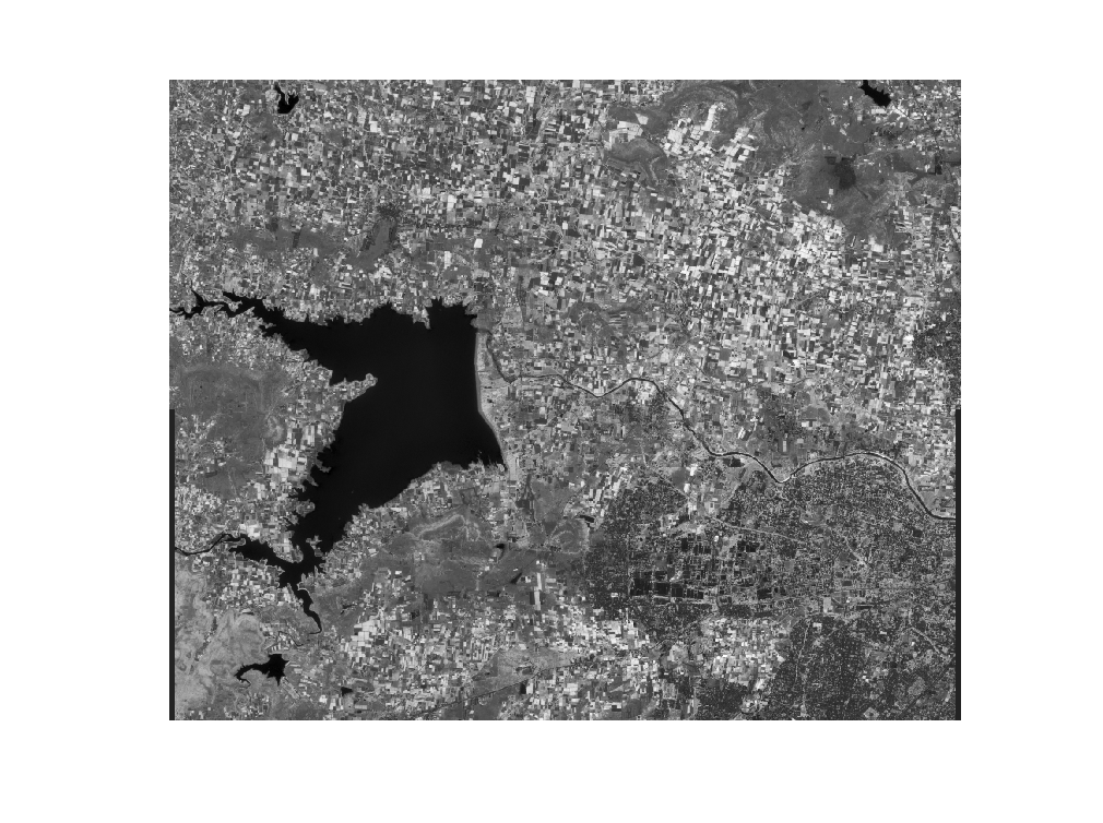
src_files = ["/content/Tiff_1.tif", "/content/Tiff_2.tif"]
srcs = [rasterio.open(p) for p in src_files]
mosaic, out_transform = merge(srcs)
out_meta = srcs[0].meta.copy()
out_meta.update({"height": mosaic.shape[1], "width": mosaic.shape[2], "transform": out_transform})
for s in srcs:
s.close()
with rasterio.open("/content/Tiff_merge.tif", "w", **out_meta) as dst:
dst.write(mosaic)
Example visualization (mosaic from Tiff_1.tif and Tiff_2.tif merged with rasterio.merge.merge):
7. Resampling (resize resolution)¶
Resampling changes how pixels are aggregated or interpolated when you change the grid size (fewer or more rows/columns) while keeping (or defining) the same geographic extent. Downsampling uses fewer pixels (coarser resolution); upsampling uses more pixels (finer resolution). Pick a method that matches your data: average or mode often suit downsampling continuous or categorical rasters; bilinear is common for smooth continuous surfaces; nearest preserves class codes when upsampling labels.
Read at a new resolution, then write a GeoTIFF with an updated affine transform so the file stays correctly georeferenced:
import rasterio
from rasterio.enums import Resampling
from rasterio.transform import Affine

src_path = "/content/Tiff_1.tif"
dst_path = "/content/Tiff_1_resampled.tif"
factor = 2  # >1 = downsample, <1 = upsample

with rasterio.open(src_path) as src:
    # New dimensions
    new_height = int(src.height / factor)
    new_width = int(src.width / factor)

    # Read & resample
    data = src.read(
        out_shape=(src.count, new_height, new_width),
        resampling=Resampling.average
    )

    # Update transform
    transform = src.transform * Affine.scale(
        src.width / new_width,
        src.height / new_height
    )

    # Update metadata
    profile = src.profile
    profile.update({
        "height": new_height,
        "width": new_width,
        "transform": transform
    })

# Save output
with rasterio.open(dst_path, "w", **profile) as dst:
    dst.write(data)

print(f"Resampled: {src.height}x{src.width} → {new_height}x{new_width}")
Example visualization (pixel grid before and after resampling Tiff_1.tif with a downsampling factor, same idea as the code above):
![]()
![]()
For upsampling (more pixels), set factor between 0 and 1 (for example factor = 0.5 doubles rows and columns) and consider Resampling.bilinear instead of average. For warping to another CRS or bounds, use rasterio.warp.reproject with a destination array and transform from calculate_default_transform (covered in more detail later in this module).
Basics assignment: GeoTIFFs & rasterio¶
These tasks recap the short recipes above: open a raster, read metadata and arrays, summarize values, plot one band, filter by value, merge two tiles, resample, and sanity-check in a viewer. Use the bundled assets/tiff/Tiff_1.tif and assets/tiff/Tiff_2.tif (see the Sample GeoTIFFs download buttons in Raster file formats). On Colab, copy the files to /content/ and change paths accordingly.
Paths
From a notebook whose working directory is the repo root, assets/tiff/Tiff_1.tif resolves like the rest of this chapter. If you run from docs/, use assets/tiff/... the same way as in 05_visualization.md.
-
Open and describe — With
rasterio.open, printsrc.shape,src.crs,src.dtypes, andsrc.boundsforTiff_1.tif. In one sentence, say whethershapeis(bands, height, width)or(height, width)in yourrasterioversion and what that implies forread(1). -
Band statistics — Read band 1 into a NumPy array (float). If
src.nodatais set, mask it tonp.nanbefore stats. Print min, max, mean (usingnp.nanmin/np.nanmax/np.nanmeanas needed). -
Quick map — Plot band 1 with
matplotlib.pyplot.imshow, passingextent=[left, right, bottom, top]fromsrc.boundsandorigin="upper". Label x / y with the axis names implied by your CRS (e.g. lon/lat for EPSG:4326). -
Value filter — Build a boolean mask that keeps pixels between the 10th and 90th percentile of the band (see § Filter pixels). Write a new GeoTIFF
Tiff_1_filtered.tif(or any output name your instructor specifies) with the same CRS/transform logic as the recipe. -
Merge — Use
rasterio.merge.mergeonTiff_1.tifandTiff_2.tif. SaveTiff_merge_lab.tif. Print the mosaic shape and confirmout_transformdiffers from either source’s transform. -
Resample — Downsample
Tiff_1.tifby factor 2 usingread(..., out_shape=..., resampling=Resampling.average)(or the Affine-scaling pattern in § Resampling). SaveTiff_1_half.tifand print before vs after width and height. -
Optional clip — Use
rasterio.mask.maskwith the inline GeoJSON box from § Clip a raster (or your own polygon in WGS 84 that intersects the raster). SaveTiff_1_clipped_lab.tif. -
Visual check — Upload
Tiff_1.tif(or your merged output) to the Pozyx Online GeoTIFF Viewer or open in QGIS. Note one thing you see thatimshowalone did not emphasize (e.g. basemap context, legend, scale).
Submit your output GeoTIFFs (or paths in a shared drive), your .py or .ipynb, and short answers for any “explain” prompts your instructor assigns.
Advance Analytics¶
The sections below use a longer teaching workflow (environment setup through practice problems). If you have not worked through the Basics assignment yet, consider doing that first so rasterio, numpy, and matplotlib patterns are fresh.
Setting Up the Environment¶
import rasterio
import rasterio.plot
import rasterio.mask
import numpy as np
import matplotlib.pyplot as plt
import geopandas as gpd
from rasterio.warp import calculate_default_transform, reproject, Resampling
from rasterio.windows import from_bounds
import warnings
warnings.filterwarnings('ignore')

# Set up plotting
plt.style.use('default')

# Data directory path - change this if your TIFF files are in a different folder
DATA_DIR = 'data/'

# Load available raster data
dem_path = DATA_DIR + 'dem.tif'
b04_path = DATA_DIR + 'B04.tif'  # Red band
b08_path = DATA_DIR + 'B08.tif'  # NIR band
true_color_path = DATA_DIR + 'true_color.tiff'

print("=== LOADING RASTER DATA ===")
print(f"DEM: {dem_path}")
print(f"Red Band (B04): {b04_path}")
print(f"NIR Band (B08): {b08_path}")
print(f"True Color: {true_color_path}")
1. Understanding Raster Structure¶
Raster Components Deep Dive¶
graph LR
    A[Raster Dataset] --> B[Metadata]
    A --> C[Data Array]
    B --> D[CRS]
    B --> E[Transform]
    B --> F[Dimensions]
    B --> G[NoData Value]
    C --> H[Pixel Values]
    C --> I[Data Type]
Metadata contains crucial information about the raster:
- CRS (Coordinate Reference System): Defines the spatial reference
- Transform: Mathematical relationship between pixel coordinates and geographic coordinates
- Dimensions: Number of rows, columns, and bands
- NoData Value: Represents missing or invalid data
Data Array holds the actual pixel values:
- Data Type: Integer (int16, int32) or floating-point (float32, float64)
- Bit Depth: Determines value range (8-bit: 0-255, 16-bit: 0-65535)
- Signed vs Unsigned: Whether negative values are allowed
Understanding the Affine Transform¶
The affine transform is a 6-parameter mathematical transformation that converts pixel coordinates to geographic coordinates:
Where:
- a: Pixel width (x-direction)
- b: Row rotation (usually 0)
- c: X-coordinate of upper-left corner
- d: Column rotation (usually 0)
- e: Pixel height (y-direction, usually negative)
- f: Y-coordinate of upper-left corner
Pixel Indexing and Coordinates¶
Pixel Coordinates: Array indices (row, column) starting from (0,0) at top-left
Geographic Coordinates: Real-world coordinates (X, Y) in the raster's CRS
Center vs Corner: Pixels can be referenced by their center point or corner
Data Types and Memory Considerations¶
| Data Type | Range | Memory per Pixel | Best Use |
|---|---|---|---|
| uint8 | 0-255 | 1 byte | Classified data, RGB images |
| int16 | -32,768 to 32,767 | 2 bytes | Elevation, temperature |
| uint16 | 0-65,535 | 2 bytes | Satellite imagery |
| float32 | ±3.4 × 10³⁸ | 4 bytes | Calculated values, ratios |
| float64 | ±1.8 × 10³⁰⁸ | 8 bytes | High-precision calculations |
Loading Real Raster Data¶
# Load the DEM (Digital Elevation Model)
with rasterio.open(dem_path) as dem_src:
    elevation_data = dem_src.read(1)  # Read first band
    dem_transform = dem_src.transform
    dem_crs = dem_src.crs
    dem_bounds = dem_src.bounds
    dem_nodata = dem_src.nodata

print("=== DEM DATA PROPERTIES ===")
print(f"Shape: {elevation_data.shape}")
print(f"Data type: {elevation_data.dtype}")
print(f"CRS: {dem_crs}")
print(f"Bounds: {dem_bounds}")
print(f"NoData value: {dem_nodata}")

# Handle NoData values
if dem_nodata is not None:
    elevation_masked = np.ma.masked_equal(elevation_data, dem_nodata)
    print(f"Valid pixels: {elevation_masked.count():,}")
    print(f"NoData pixels: {elevation_masked.mask.sum():,}")
    # Use masked array for statistics
    print(f"Min elevation: {elevation_masked.min():.1f}m")
    print(f"Max elevation: {elevation_masked.max():.1f}m")
    print(f"Mean elevation: {elevation_masked.mean():.1f}m")
else:
    print(f"Min elevation: {elevation_data.min():.1f}m")
    print(f"Max elevation: {elevation_data.max():.1f}m")
    print(f"Mean elevation: {elevation_data.mean():.1f}m")
Raster Metadata and Transform¶
# Use the actual transform from the DEM
transform = dem_transform
bounds = dem_bounds
height, width = elevation_data.shape

print("=== RASTER SPATIAL PROPERTIES ===")
print(f"Bounds: {bounds}")
print(f"Transform: {transform}")
print(f"Pixel size X: {transform[0]:.4f}")
print(f"Pixel size Y: {abs(transform[4]):.4f}")
print(f"Width: {width} pixels")
print(f"Height: {height} pixels")

# Calculate pixel coordinates
def pixel_to_coord(row, col, transform):
    """Convert pixel coordinates to geographic coordinates"""
    x = transform[0] * col + transform[1] * row + transform[2]
    y = transform[3] * col + transform[4] * row + transform[5]
    return x, y

# Example: center pixel coordinates
center_row, center_col = height // 2, width // 2
center_x, center_y = pixel_to_coord(center_row, center_col, transform)
print(f"Center pixel ({center_row}, {center_col}) = ({center_x:.2f}, {center_y:.2f})")

# Calculate extent for plotting
extent = [bounds.left, bounds.right, bounds.bottom, bounds.top]
print(f"Plot extent: {extent}")
2. Visualizing Raster Data¶
Basic Raster Visualization¶
# Create comprehensive visualization
fig, axes = plt.subplots(2, 2, figsize=(15, 12))

# 1. Basic elevation map
im1 = axes[0,0].imshow(elevation_data, cmap='terrain', extent=bounds)
axes[0,0].set_title('Elevation Map')
axes[0,0].set_xlabel('Longitude')
axes[0,0].set_ylabel('Latitude')
plt.colorbar(im1, ax=axes[0,0], label='Elevation (m)')

# 2. Hillshade effect
from matplotlib.colors import LightSource
ls = LightSource(azdeg=315, altdeg=45)
hillshade = ls.hillshade(elevation_data, vert_exag=2)
axes[0,1].imshow(hillshade, cmap='gray', extent=bounds)
axes[0,1].set_title('Hillshade')
axes[0,1].set_xlabel('Longitude')
axes[0,1].set_ylabel('Latitude')

# 3. Elevation histogram
axes[1,0].hist(elevation_data.flatten(), bins=50, alpha=0.7, color='brown')
axes[1,0].set_title('Elevation Distribution')
axes[1,0].set_xlabel('Elevation (m)')
axes[1,0].set_ylabel('Frequency')
axes[1,0].grid(True, alpha=0.3)

# 4. Contour lines
contour = axes[1,1].contour(elevation_data, levels=10, extent=bounds, colors='black', alpha=0.6)
axes[1,1].clabel(contour, inline=True, fontsize=8)
im4 = axes[1,1].imshow(elevation_data, cmap='terrain', extent=bounds, alpha=0.7)
axes[1,1].set_title('Elevation with Contours')
axes[1,1].set_xlabel('Longitude')
axes[1,1].set_ylabel('Latitude')

plt.tight_layout()
plt.show()
Advanced Visualization Techniques¶
# Create elevation classes
def classify_elevation(elevation, breaks):
    """Classify elevation into categories"""
    classified = np.zeros_like(elevation, dtype=np.int32)
    for i, break_val in enumerate(breaks[1:], 1):
        classified[elevation <= break_val] = i
    return classified

# Define elevation breaks
elevation_breaks = [0, 200, 500, 800, 1200, 2000]
elevation_classes = classify_elevation(elevation_data, elevation_breaks)

# Create custom colormap
colors = ['#2E8B57', '#9ACD32', '#DAA520', '#CD853F', '#A0522D', '#FFFFFF']
from matplotlib.colors import ListedColormap
custom_cmap = ListedColormap(colors[:len(elevation_breaks)-1])

# Plot classified elevation
fig, (ax1, ax2) = plt.subplots(1, 2, figsize=(15, 6))

# Original continuous elevation
im1 = ax1.imshow(elevation_data, cmap='terrain', extent=bounds)
ax1.set_title('Continuous Elevation')
plt.colorbar(im1, ax=ax1, label='Elevation (m)')

# Classified elevation
im2 = ax2.imshow(elevation_classes, cmap=custom_cmap, extent=bounds)
ax2.set_title('Classified Elevation')
cbar = plt.colorbar(im2, ax=ax2, ticks=range(len(elevation_breaks)-1))
cbar.set_ticklabels([f'{elevation_breaks[i]}-{elevation_breaks[i+1]}m'
                     for i in range(len(elevation_breaks)-1)])

plt.tight_layout()
plt.show()
3. Raster Calculations and Statistics¶
Basic Statistics¶
# Calculate comprehensive statistics
def raster_statistics(data, name="Raster"):
    """Calculate comprehensive raster statistics"""
    # Remove any potential NoData values (assuming -9999)
    valid_data = data[data != -9999]

    stats = {
        'count': valid_data.size,
        'min': valid_data.min(),
        'max': valid_data.max(),
        'mean': valid_data.mean(),
        'median': np.median(valid_data),
        'std': valid_data.std(),
        'range': valid_data.max() - valid_data.min()
    }

    print(f"=== {name.upper()} STATISTICS ===")
    for key, value in stats.items():
        if key == 'count':
            print(f"{key.capitalize()}: {value:,}")
        else:
            print(f"{key.capitalize()}: {value:.2f}")

    return stats

# Calculate statistics for our elevation data
elev_stats = raster_statistics(elevation_data, "Elevation")

# Percentiles
percentiles = [10, 25, 50, 75, 90, 95, 99]
elev_percentiles = np.percentile(elevation_data, percentiles)

print(f"\n=== ELEVATION PERCENTILES ===")
for p, val in zip(percentiles, elev_percentiles):
    print(f"{p}th percentile: {val:.1f}m")
Raster Math Operations¶
# Demonstrate various raster calculations
print("=== RASTER CALCULATIONS ===")

# 1. Convert elevation to feet
elevation_feet = elevation_data * 3.28084
print(f"Elevation in feet - Min: {elevation_feet.min():.1f}, Max: {elevation_feet.max():.1f}")

# 2. Calculate slope (simplified)
def calculate_slope(elevation, pixel_size):
    """Calculate slope using gradient"""
    grad_y, grad_x = np.gradient(elevation, pixel_size)
    slope_radians = np.arctan(np.sqrt(grad_x**2 + grad_y**2))
    slope_degrees = np.degrees(slope_radians)
    return slope_degrees

pixel_size = abs(transform[0])  # Assuming square pixels
slope_data = calculate_slope(elevation_data, pixel_size)

print(f"Slope - Min: {slope_data.min():.1f}°, Max: {slope_data.max():.1f}°, Mean: {slope_data.mean():.1f}°")

# 3. Create binary mask (high elevation areas)
high_elevation_mask = elevation_data > np.percentile(elevation_data, 75)
high_elevation_area = np.sum(high_elevation_mask) * (pixel_size ** 2)

print(f"High elevation areas (>75th percentile): {high_elevation_area:.2f} square units")

# 4. Normalize elevation (0-1 scale)
elevation_normalized = (elevation_data - elevation_data.min()) / (elevation_data.max() - elevation_data.min())
print(f"Normalized elevation - Min: {elevation_normalized.min():.3f}, Max: {elevation_normalized.max():.3f}")
Visualizing Calculated Rasters¶
# Visualize calculated rasters
fig, axes = plt.subplots(2, 2, figsize=(15, 12))

# Original elevation
im1 = axes[0,0].imshow(elevation_data, cmap='terrain', extent=bounds)
axes[0,0].set_title('Original Elevation')
plt.colorbar(im1, ax=axes[0,0], label='Elevation (m)')

# Slope
im2 = axes[0,1].imshow(slope_data, cmap='Reds', extent=bounds)
axes[0,1].set_title('Slope')
plt.colorbar(im2, ax=axes[0,1], label='Slope (degrees)')

# High elevation mask
im3 = axes[1,0].imshow(high_elevation_mask, cmap='RdYlBu_r', extent=bounds)
axes[1,0].set_title('High Elevation Areas (>75th percentile)')
plt.colorbar(im3, ax=axes[1,0], label='High Elevation')

# Normalized elevation
im4 = axes[1,1].imshow(elevation_normalized, cmap='viridis', extent=bounds)
axes[1,1].set_title('Normalized Elevation (0-1)')
plt.colorbar(im4, ax=axes[1,1], label='Normalized Value')

plt.tight_layout()
plt.show()
4. Working with Vector Boundaries¶
Creating Sample Vector Data¶
# Create sample vector boundaries for clipping
from shapely.geometry import Polygon, Point
import geopandas as gpd

# Create sample study areas
study_areas = [
    {'name': 'Area A', 'geometry': Polygon([(-5, -5), (0, -5), (0, 0), (-5, 0), (-5, -5)])},
    {'name': 'Area B', 'geometry': Polygon([(2, 2), (8, 2), (8, 8), (2, 8), (2, 2)])},
    {'name': 'Circular Area', 'geometry': Point(3, -3).buffer(3)}
]

study_gdf = gpd.GeoDataFrame(study_areas, crs='EPSG:4326')

print("=== STUDY AREAS ===")
print(study_gdf)

# Visualize study areas with elevation
fig, ax = plt.subplots(1, 1, figsize=(12, 10))

# Plot elevation as background
im = ax.imshow(elevation_data, cmap='terrain', extent=bounds, alpha=0.7)
plt.colorbar(im, ax=ax, label='Elevation (m)')

# Plot study areas
study_gdf.plot(ax=ax, facecolor='none', edgecolor='red', linewidth=3, alpha=0.8)

# Add labels
for idx, row in study_gdf.iterrows():
    centroid = row.geometry.centroid
    ax.annotate(row['name'], (centroid.x, centroid.y),
                ha='center', va='center', fontsize=12, fontweight='bold',
                bbox=dict(boxstyle='round,pad=0.3', facecolor='white', alpha=0.8))

ax.set_title('Study Areas on Elevation Map')
ax.set_xlabel('Longitude')
ax.set_ylabel('Latitude')
plt.tight_layout()
plt.show()
Clipping Rasters with Vector Boundaries¶
def clip_raster_with_polygon(raster_data, transform, polygon, bounds):
    """Clip raster data using a polygon boundary"""
    from rasterio.features import geometry_mask

    # Create mask from polygon
    mask = geometry_mask([polygon], transform=transform,
                        invert=True, out_shape=raster_data.shape)

    # Apply mask
    clipped_data = raster_data.copy()
    clipped_data[~mask] = np.nan  # Set areas outside polygon to NaN

    return clipped_data, mask

# Clip elevation data for each study area
clipped_results = {}

for idx, area in study_gdf.iterrows():
    clipped_elev, mask = clip_raster_with_polygon(
        elevation_data, transform, area.geometry, bounds
    )
    clipped_results[area['name']] = {
        'data': clipped_elev,
        'mask': mask,
        'geometry': area.geometry
    }

# Visualize clipped results
fig, axes = plt.subplots(2, 2, figsize=(15, 12))
axes = axes.flatten()

# Original elevation
im0 = axes[0].imshow(elevation_data, cmap='terrain', extent=bounds)
study_gdf.plot(ax=axes[0], facecolor='none', edgecolor='red', linewidth=2)
axes[0].set_title('Original Elevation with Study Areas')
plt.colorbar(im0, ax=axes[0], label='Elevation (m)')

# Clipped areas
for i, (name, result) in enumerate(clipped_results.items(), 1):
    if i < 4:  # Only plot first 3 clipped areas
        im = axes[i].imshow(result['data'], cmap='terrain', extent=bounds)
        axes[i].set_title(f'Clipped Elevation - {name}')
        plt.colorbar(im, ax=axes[i], label='Elevation (m)')

plt.tight_layout()
plt.show()
Statistics for Clipped Areas¶
# Calculate statistics for each clipped area
print("=== CLIPPED AREA STATISTICS ===")

for name, result in clipped_results.items():
    clipped_data = result['data']
    valid_data = clipped_data[~np.isnan(clipped_data)]

    if len(valid_data) > 0:
        print(f"\n{name}:")
        print(f"  Valid pixels: {len(valid_data):,}")
        print(f"  Min elevation: {valid_data.min():.1f}m")
        print(f"  Max elevation: {valid_data.max():.1f}m")
        print(f"  Mean elevation: {valid_data.mean():.1f}m")
        print(f"  Std deviation: {valid_data.std():.1f}m")

        # Calculate area (assuming each pixel represents area)
        pixel_area = (pixel_size ** 2)
        total_area = len(valid_data) * pixel_area
        print(f"  Total area: {total_area:.2f} square units")
    else:
        print(f"\n{name}: No valid data")
5. Raster-Vector Integration¶
Extracting Values at Points¶
# Create sample point locations
sample_points = [
    {'name': 'Peak A', 'geometry': Point(-2, 3)},
    {'name': 'Valley B', 'geometry': Point(4, -2)},
    {'name': 'Ridge C', 'geometry': Point(-6, -1)},
    {'name': 'Plain D', 'geometry': Point(7, 5)}
]

points_gdf = gpd.GeoDataFrame(sample_points, crs='EPSG:4326')

def extract_raster_values_at_points(raster_data, transform, points_gdf):
    """Extract raster values at point locations"""
    from rasterio.transform import rowcol

    extracted_values = []

    for idx, point in points_gdf.iterrows():
        # Convert geographic coordinates to pixel coordinates
        row, col = rowcol(transform, point.geometry.x, point.geometry.y)

        # Check if point is within raster bounds
        if 0 <= row < raster_data.shape[0] and 0 <= col < raster_data.shape[1]:
            value = raster_data[row, col]
            extracted_values.append(value)
        else:
            extracted_values.append(np.nan)

    return extracted_values

# Extract elevation values at points
elevation_at_points = extract_raster_values_at_points(elevation_data, transform, points_gdf)
slope_at_points = extract_raster_values_at_points(slope_data, transform, points_gdf)

# Add values to GeoDataFrame
points_gdf['elevation'] = elevation_at_points
points_gdf['slope'] = slope_at_points

print("=== ELEVATION AND SLOPE AT SAMPLE POINTS ===")
print(points_gdf[['name', 'elevation', 'slope']])

# Visualize points on raster
fig, (ax1, ax2) = plt.subplots(1, 2, figsize=(15, 6))

# Elevation with points
im1 = ax1.imshow(elevation_data, cmap='terrain', extent=bounds)
points_gdf.plot(ax=ax1, color='red', markersize=100, marker='*', edgecolor='black', linewidth=1)
for idx, point in points_gdf.iterrows():
    ax1.annotate(f"{point['name']}\n{point['elevation']:.0f}m",
                (point.geometry.x, point.geometry.y),
                xytext=(10, 10), textcoords='offset points',
                bbox=dict(boxstyle='round,pad=0.3', facecolor='white', alpha=0.8),
                fontsize=8)
ax1.set_title('Elevation Values at Sample Points')
plt.colorbar(im1, ax=ax1, label='Elevation (m)')

# Slope with points
im2 = ax2.imshow(slope_data, cmap='Reds', extent=bounds)
points_gdf.plot(ax=ax2, color='blue', markersize=100, marker='*', edgecolor='black', linewidth=1)
for idx, point in points_gdf.iterrows():
    ax2.annotate(f"{point['name']}\n{point['slope']:.1f}°",
                (point.geometry.x, point.geometry.y),
                xytext=(10, 10), textcoords='offset points',
                bbox=dict(boxstyle='round,pad=0.3', facecolor='white', alpha=0.8),
                fontsize=8)
ax2.set_title('Slope Values at Sample Points')
plt.colorbar(im2, ax=ax2, label='Slope (degrees)')

plt.tight_layout()
plt.show()
Zonal Statistics¶
def calculate_zonal_statistics(raster_data, zones_gdf, transform):
    """Calculate statistics for each zone (polygon)"""
    from rasterio.features import geometry_mask

    results = []

    for idx, zone in zones_gdf.iterrows():
        # Create mask for this zone
        mask = geometry_mask([zone.geometry], transform=transform,
                           invert=True, out_shape=raster_data.shape)

        # Extract values within zone
        zone_values = raster_data[mask]
        zone_values = zone_values[~np.isnan(zone_values)]  # Remove NaN values

        if len(zone_values) > 0:
            stats = {
                'zone_name': zone.get('name', f'Zone_{idx}'),
                'count': len(zone_values),
                'min': zone_values.min(),
                'max': zone_values.max(),
                'mean': zone_values.mean(),
                'median': np.median(zone_values),
                'std': zone_values.std(),
                'sum': zone_values.sum()
            }
        else:
            stats = {
                'zone_name': zone.get('name', f'Zone_{idx}'),
                'count': 0,
                'min': np.nan,
                'max': np.nan,
                'mean': np.nan,
                'median': np.nan,
                'std': np.nan,
                'sum': np.nan
            }

        results.append(stats)

    return pd.DataFrame(results)

# Calculate zonal statistics for elevation
zonal_stats = calculate_zonal_statistics(elevation_data, study_gdf, transform)

print("=== ZONAL STATISTICS FOR ELEVATION ===")
print(zonal_stats.round(2))

# Calculate zonal statistics for slope
slope_zonal_stats = calculate_zonal_statistics(slope_data, study_gdf, transform)

print("\n=== ZONAL STATISTICS FOR SLOPE ===")
print(slope_zonal_stats.round(2))
7. Multi-band Raster Analysis¶
NDVI Calculation from Two Bands¶
NDVI (Normalized Difference Vegetation Index) is calculated using Near-Infrared (NIR) and Red bands to assess vegetation health.
# Load the satellite bands
with rasterio.open(b08_path) as nir_src:
    nir_data = nir_src.read(1).astype(float)  # NIR band (B08)
    nir_transform = nir_src.transform
    nir_bounds = nir_src.bounds
    nir_nodata = nir_src.nodata

with rasterio.open(b04_path) as red_src:
    red_data = red_src.read(1).astype(float)  # Red band (B04)
    red_transform = red_src.transform
    red_bounds = red_src.bounds
    red_nodata = red_src.nodata

print("=== SATELLITE BAND DATA ===")
print(f"NIR Band shape: {nir_data.shape}")
print(f"Red Band shape: {red_data.shape}")
print(f"NIR range: {nir_data.min():.0f} - {nir_data.max():.0f}")
print(f"Red range: {red_data.min():.0f} - {red_data.max():.0f}")
print(f"NIR NoData: {nir_nodata}")
print(f"Red NoData: {red_nodata}")

# Handle NoData values and convert to reflectance (0-1 scale)
if nir_nodata is not None:
    nir_data = np.where(nir_data == nir_nodata, np.nan, nir_data)
if red_nodata is not None:
    red_data = np.where(red_data == red_nodata, np.nan, red_data)

# Convert to reflectance if needed (assuming values are in 0-10000 range)
if nir_data.max() > 1:
    nir_data = nir_data / 10000.0
if red_data.max() > 1:
    red_data = red_data / 10000.0

print(f"NIR reflectance range: {np.nanmin(nir_data):.3f} - {np.nanmax(nir_data):.3f}")
print(f"Red reflectance range: {np.nanmin(red_data):.3f} - {np.nanmax(red_data):.3f}")

# Calculate NDVI
def calculate_ndvi(nir, red):
    """Calculate NDVI from NIR and Red bands"""
    # Avoid division by zero
    denominator = nir + red
    ndvi = np.where(denominator != 0, (nir - red) / denominator, np.nan)
    return ndvi

ndvi = calculate_ndvi(nir_data, red_data)

print(f"\nNDVI range: {np.nanmin(ndvi):.3f} - {np.nanmax(ndvi):.3f}")
print(f"Mean NDVI: {np.nanmean(ndvi):.3f}")

# Calculate extent for plotting
band_extent = [nir_bounds.left, nir_bounds.right, nir_bounds.bottom, nir_bounds.top]

# Visualize bands and NDVI
fig, axes = plt.subplots(2, 2, figsize=(15, 12))

# NIR Band
im1 = axes[0,0].imshow(nir_data, cmap='Reds', extent=band_extent)
axes[0,0].set_title('NIR Band (B08)')
plt.colorbar(im1, ax=axes[0,0], label='Reflectance')

# Red Band
im2 = axes[0,1].imshow(red_data, cmap='Reds', extent=band_extent)
axes[0,1].set_title('Red Band (B04)')
plt.colorbar(im2, ax=axes[0,1], label='Reflectance')

# NDVI
im3 = axes[1,0].imshow(ndvi, cmap='RdYlGn', vmin=-1, vmax=1, extent=band_extent)
axes[1,0].set_title('NDVI (Vegetation Index)')
plt.colorbar(im3, ax=axes[1,0], label='NDVI Value')

# NDVI Classification
ndvi_classes = np.where(ndvi < 0, 0,      # Water/bare soil
                np.where(ndvi < 0.2, 1,   # Low vegetation
                np.where(ndvi < 0.5, 2,   # Moderate vegetation
                         3)))             # High vegetation

class_colors = ['blue', 'brown', 'yellow', 'green']
class_labels = ['Water/Bare', 'Low Veg', 'Moderate Veg', 'High Veg']
from matplotlib.colors import ListedColormap
class_cmap = ListedColormap(class_colors)

im4 = axes[1,1].imshow(ndvi_classes, cmap=class_cmap, extent=band_extent)
axes[1,1].set_title('NDVI Classification')
cbar = plt.colorbar(im4, ax=axes[1,1], ticks=[0, 1, 2, 3])
cbar.set_ticklabels(class_labels)

plt.tight_layout()
plt.show()

# NDVI Statistics
print("\n=== NDVI ANALYSIS ===")
for i, label in enumerate(class_labels):
    pixel_count = np.sum(ndvi_classes == i)
    percentage = (pixel_count / ndvi_classes.size) * 100
    print(f"{label}: {pixel_count:,} pixels ({percentage:.1f}%)")
RGB Visualization from Three Bands¶
True Color Composite uses Red, Green, and Blue bands to create natural-looking images.
# Load the true color composite
with rasterio.open(true_color_path) as rgb_src:
    rgb_data = rgb_src.read()  # Read all bands
    rgb_transform = rgb_src.transform
    rgb_bounds = rgb_src.bounds
    rgb_nodata = rgb_src.nodata

print("=== TRUE COLOR COMPOSITE DATA ===")
print(f"RGB data shape: {rgb_data.shape}")
print(f"Number of bands: {rgb_data.shape[0]}")
print(f"Image dimensions: {rgb_data.shape[1]} x {rgb_data.shape[2]}")
print(f"Data type: {rgb_data.dtype}")
print(f"NoData value: {rgb_nodata}")

# Handle the data for visualization
if rgb_data.shape[0] >= 3:
    # Extract RGB bands (assuming order is R, G, B)
    red_band = rgb_data[0].astype(float)
    green_band = rgb_data[1].astype(float)
    blue_band = rgb_data[2].astype(float)

    # Handle NoData values
    if rgb_nodata is not None:
        red_band = np.where(red_band == rgb_nodata, np.nan, red_band)
        green_band = np.where(green_band == rgb_nodata, np.nan, green_band)
        blue_band = np.where(blue_band == rgb_nodata, np.nan, blue_band)

    print(f"Red band range: {np.nanmin(red_band):.0f} - {np.nanmax(red_band):.0f}")
    print(f"Green band range: {np.nanmin(green_band):.0f} - {np.nanmax(green_band):.0f}")
    print(f"Blue band range: {np.nanmin(blue_band):.0f} - {np.nanmax(blue_band):.0f}")

    # Create RGB composite
    def create_rgb_composite(red, green, blue, enhance=True):
        """Create RGB composite from three bands"""
        # Normalize to 0-1 range if needed
        if red.max() > 1:
            red = red / np.nanmax(red)
        if green.max() > 1:
            green = green / np.nanmax(green)
        if blue.max() > 1:
            blue = blue / np.nanmax(blue)

        # Stack bands into 3D array
        rgb = np.dstack((red, green, blue))

        if enhance:
            # Enhance contrast (stretch to full 0-1 range)
            for i in range(3):
                band = rgb[:, :, i]
                band_min, band_max = np.nanmin(band), np.nanmax(band)
                if band_max > band_min:
                    rgb[:, :, i] = (band - band_min) / (band_max - band_min)

        return rgb

    # Create composites
    rgb_natural = create_rgb_composite(red_band, green_band, blue_band, enhance=False)
    rgb_enhanced = create_rgb_composite(red_band, green_band, blue_band, enhance=True)

    # Calculate extent for plotting
    rgb_extent = [rgb_bounds.left, rgb_bounds.right, rgb_bounds.bottom, rgb_bounds.top]

    # Visualize individual bands and composites
    fig, axes = plt.subplots(2, 3, figsize=(18, 12))

    # Individual bands
    im1 = axes[0,0].imshow(red_band, cmap='Reds', extent=rgb_extent)
    axes[0,0].set_title('Red Band')
    plt.colorbar(im1, ax=axes[0,0], label='Digital Number')

    im2 = axes[0,1].imshow(green_band, cmap='Greens', extent=rgb_extent)
    axes[0,1].set_title('Green Band')
    plt.colorbar(im2, ax=axes[0,1], label='Digital Number')

    im3 = axes[0,2].imshow(blue_band, cmap='Blues', extent=rgb_extent)
    axes[0,2].set_title('Blue Band')
    plt.colorbar(im3, ax=axes[0,2], label='Digital Number')

    # RGB composites
    axes[1,0].imshow(rgb_natural, extent=rgb_extent)
    axes[1,0].set_title('Natural Color Composite')

    axes[1,1].imshow(rgb_enhanced, extent=rgb_extent)
    axes[1,1].set_title('Enhanced Color Composite')

    # False color composite (NIR-Red-Green) if NIR data is available
    if 'nir_data' in locals() and nir_data.shape == red_band.shape:
        false_color = create_rgb_composite(nir_data, red_band, green_band)
        axes[1,2].imshow(false_color, extent=rgb_extent)
        axes[1,2].set_title('False Color Composite\n(NIR-Red-Green)')
    else:
        axes[1,2].text(0.5, 0.5, 'NIR data not available\nfor false color composite',
                      ha='center', va='center', transform=axes[1,2].transAxes)
        axes[1,2].set_title('False Color Composite\n(Not Available)')

    plt.tight_layout()
    plt.show()

    # Band statistics
    print("\n=== BAND STATISTICS ===")
    bands = {'Red': red_band, 'Green': green_band, 'Blue': blue_band}
    if 'nir_data' in locals():
        bands['NIR'] = nir_data

    for band_name, band_data in bands.items():
        print(f"{band_name} Band:")
        print(f"  Mean: {np.nanmean(band_data):.1f}")
        print(f"  Std:  {np.nanstd(band_data):.1f}")
        print(f"  Min:  {np.nanmin(band_data):.1f}")
        print(f"  Max:  {np.nanmax(band_data):.1f}")
else:
    print("Error: True color composite does not have enough bands for RGB visualization")
8. Handling NoData Values¶
# Create sample data with NoData values
elevation_with_nodata = elevation_data.copy()

# Introduce some NoData areas (simulate missing data)
# Set random patches to NoData value (-9999)
nodata_value = -9999
np.random.seed(42)  # For reproducible results

# Create random NoData patches
for _ in range(5):
    center_row = np.random.randint(20, elevation_data.shape[0] - 20)
    center_col = np.random.randint(20, elevation_data.shape[1] - 20)
    size = np.random.randint(5, 15)

    elevation_with_nodata[
        center_row-size:center_row+size,
        center_col-size:center_col+size
    ] = nodata_value

print("=== NODATA HANDLING ===")
print(f"Original data shape: {elevation_data.shape}")
print(f"NoData value: {nodata_value}")
print(f"Number of NoData pixels: {np.sum(elevation_with_nodata == nodata_value)}")
print(f"Percentage NoData: {np.sum(elevation_with_nodata == nodata_value) / elevation_with_nodata.size * 100:.1f}%")

# Create masked array for proper handling
elevation_masked = np.ma.masked_equal(elevation_with_nodata, nodata_value)

print(f"Valid data points: {elevation_masked.count()}")
print(f"Masked data points: {elevation_masked.mask.sum()}")
NoData Visualization and Statistics¶
# Visualize data with NoData
fig, axes = plt.subplots(1, 3, figsize=(18, 6))

# Original data
im1 = axes[0].imshow(elevation_data, cmap='terrain', extent=bounds)
axes[0].set_title('Original Elevation Data')
plt.colorbar(im1, ax=axes[0], label='Elevation (m)')

# Data with NoData (showing NoData as white)
elevation_display = elevation_with_nodata.copy()
elevation_display[elevation_display == nodata_value] = np.nan
im2 = axes[1].imshow(elevation_display, cmap='terrain', extent=bounds)
axes[1].set_title('Elevation Data with NoData (white areas)')
plt.colorbar(im2, ax=axes[1], label='Elevation (m)')

# NoData mask only
nodata_mask = elevation_with_nodata == nodata_value
im3 = axes[2].imshow(nodata_mask, cmap='RdYlBu_r', extent=bounds)
axes[2].set_title('NoData Mask (red = NoData)')
plt.colorbar(im3, ax=axes[2], label='NoData')

plt.tight_layout()
plt.show()

# Statistics comparison
print("\n=== STATISTICS COMPARISON ===")
print("Original data:")
raster_statistics(elevation_data, "Original")

print("\nData with NoData (excluding NoData values):")
valid_data = elevation_with_nodata[elevation_with_nodata != nodata_value]
raster_statistics(valid_data, "Valid Data Only")
Filling NoData Values¶
# Demonstrate different NoData filling methods
from scipy import ndimage

def fill_nodata_methods(data, nodata_value):
    """Demonstrate different methods to fill NoData values"""
    # Create mask
    mask = data == nodata_value
    filled_data = data.copy().astype(float)
    filled_data[mask] = np.nan

    methods = {}

    # Method 1: Fill with mean
    mean_filled = filled_data.copy()
    mean_value = np.nanmean(filled_data)
    mean_filled[np.isnan(mean_filled)] = mean_value
    methods['Mean Fill'] = mean_filled

    # Method 2: Fill with median
    median_filled = filled_data.copy()
    median_value = np.nanmedian(filled_data)
    median_filled[np.isnan(median_filled)] = median_value
    methods['Median Fill'] = median_filled

    # Method 3: Interpolation (simple nearest neighbor)
    from scipy.interpolate import griddata

    # Get coordinates of valid and invalid points
    rows, cols = np.mgrid[0:data.shape[0], 0:data.shape[1]]
    valid_mask = ~np.isnan(filled_data)

    if np.sum(valid_mask) > 0:
        # Interpolate
        interpolated = griddata(
            (rows[valid_mask], cols[valid_mask]),
            filled_data[valid_mask],
            (rows, cols),
            method='nearest'
        )
        methods['Nearest Neighbor'] = interpolated

    return methods

# Apply different filling methods
filled_methods = fill_nodata_methods(elevation_with_nodata, nodata_value)

# Visualize different filling methods
fig, axes = plt.subplots(2, 2, figsize=(15, 12))
axes = axes.flatten()

# Original with NoData
elevation_display = elevation_with_nodata.copy()
elevation_display[elevation_display == nodata_value] = np.nan
im0 = axes[0].imshow(elevation_display, cmap='terrain', extent=bounds)
axes[0].set_title('Original with NoData')
plt.colorbar(im0, ax=axes[0], label='Elevation (m)')

# Different filling methods
for i, (method_name, filled_data) in enumerate(filled_methods.items(), 1):
    if i < 4:
        im = axes[i].imshow(filled_data, cmap='terrain', extent=bounds)
        axes[i].set_title(f'{method_name}')
        plt.colorbar(im, ax=axes[i], label='Elevation (m)')

plt.tight_layout()
plt.show()
Practice Problems¶
Problem 1: Elevation Analysis¶
Perform comprehensive elevation analysis:
# TODO:
# 1. Create elevation zones (low, medium, high)
# 2. Calculate the area of each elevation zone
# 3. Find the steepest areas (top 10% slope)
# 4. Create a suitability map combining elevation and slope
# 5. Generate summary statistics

# Your code here
Solution
# 1. Create elevation zones
elevation_percentiles = np.percentile(elevation_data, [33, 67])
elevation_zones = np.zeros_like(elevation_data, dtype=int)
elevation_zones[elevation_data <= elevation_percentiles[0]] = 1  # Low
elevation_zones[(elevation_data > elevation_percentiles[0]) &
               (elevation_data <= elevation_percentiles[1])] = 2  # Medium
elevation_zones[elevation_data > elevation_percentiles[1]] = 3  # High

# 2. Calculate area of each zone
pixel_area = (pixel_size ** 2)
zone_areas = {}
zone_names = {1: 'Low', 2: 'Medium', 3: 'High'}

for zone_id, zone_name in zone_names.items():
    zone_pixels = np.sum(elevation_zones == zone_id)
    zone_area = zone_pixels * pixel_area
    zone_areas[zone_name] = zone_area
    print(f"{zone_name} elevation zone: {zone_pixels:,} pixels, {zone_area:.2f} sq units")

# 3. Find steepest areas (top 10% slope)
slope_threshold = np.percentile(slope_data, 90)
steep_areas = slope_data > slope_threshold
steep_area_total = np.sum(steep_areas) * pixel_area

print(f"\nSteepest areas (>{slope_threshold:.1f}°): {steep_area_total:.2f} sq units")

# 4. Create suitability map (example: suitable = medium elevation + gentle slope)
gentle_slope = slope_data < np.percentile(slope_data, 50)  # Bottom 50% slope
medium_elevation = elevation_zones == 2
suitability = (medium_elevation & gentle_slope).astype(int)

suitable_area = np.sum(suitability) * pixel_area
print(f"Suitable areas (medium elevation + gentle slope): {suitable_area:.2f} sq units")

# 5. Visualize results
fig, axes = plt.subplots(2, 2, figsize=(15, 12))

# Elevation zones
zone_colors = ['white', 'green', 'yellow', 'red']
zone_cmap = ListedColormap(zone_colors)
im1 = axes[0,0].imshow(elevation_zones, cmap=zone_cmap, extent=bounds)
axes[0,0].set_title('Elevation Zones')

# Steep areas
im2 = axes[0,1].imshow(steep_areas, cmap='Reds', extent=bounds)
axes[0,1].set_title('Steepest Areas (Top 10%)')

# Suitability map
im3 = axes[1,0].imshow(suitability, cmap='RdYlGn', extent=bounds)
axes[1,0].set_title('Suitability Map')

# Combined visualization
axes[1,1].imshow(elevation_data, cmap='terrain', extent=bounds, alpha=0.7)
axes[1,1].contour(slope_data, levels=[slope_threshold], colors='red', linewidths=2)
axes[1,1].set_title('Elevation with Steep Area Contours')

plt.tight_layout()
plt.show()
Problem 2: Multi-Criteria Analysis¶
Combine multiple raster layers for analysis:
# TODO:
# 1. Create a temperature raster (simulate climate data)
# 2. Create a distance-to-water raster (simulate accessibility)
# 3. Combine elevation, slope, temperature, and distance for habitat suitability
# 4. Apply different weights to each factor
# 5. Identify the top 20% most suitable areas

# Your code here
Solution
# 1. Create temperature raster (simulate)
x = np.linspace(-10, 10, elevation_data.shape[1])
y = np.linspace(-10, 10, elevation_data.shape[0])
X, Y = np.meshgrid(x, y)

# Temperature decreases with elevation and varies with latitude
temperature_data = (
    25 - (elevation_data / 100) +  # Temperature lapse rate
    5 * np.sin(Y / 5) +            # Latitudinal variation
    3 * np.random.random(elevation_data.shape)  # Random variation
)

# 2. Create distance-to-water raster (simulate rivers/lakes)
# Create some "water bodies" as low elevation areas
water_bodies = elevation_data < np.percentile(elevation_data, 20)

# Calculate distance to nearest water
from scipy.ndimage import distance_transform_edt
distance_to_water = distance_transform_edt(~water_bodies) * pixel_size

print("=== SIMULATED DATA CREATED ===")
print(f"Temperature range: {temperature_data.min():.1f}°C to {temperature_data.max():.1f}°C")
print(f"Distance to water range: {distance_to_water.min():.1f} to {distance_to_water.max():.1f} units")

# 3. Normalize all factors to 0-1 scale for combination
def normalize_raster(data):
    return (data - data.min()) / (data.max() - data.min())

# Normalize factors (some need to be inverted for suitability)
elev_norm = 1 - normalize_raster(np.abs(elevation_data - np.median(elevation_data)))  # Prefer medium elevation
slope_norm = 1 - normalize_raster(slope_data)  # Prefer gentle slopes
temp_norm = 1 - normalize_raster(np.abs(temperature_data - 20))  # Prefer ~20°C
water_norm = 1 - normalize_raster(distance_to_water)  # Prefer close to water

# 4. Apply weights and combine
weights = {
    'elevation': 0.3,
    'slope': 0.3,
    'temperature': 0.2,
    'water_distance': 0.2
}

habitat_suitability = (
    weights['elevation'] * elev_norm +
    weights['slope'] * slope_norm +
    weights['temperature'] * temp_norm +
    weights['water_distance'] * water_norm
)

# 5. Identify top 20% most suitable areas
suitability_threshold = np.percentile(habitat_suitability, 80)
top_suitable = habitat_suitability > suitability_threshold

suitable_area = np.sum(top_suitable) * pixel_area
total_area = habitat_suitability.size * pixel_area

print(f"\n=== HABITAT SUITABILITY RESULTS ===")
print(f"Suitability threshold (80th percentile): {suitability_threshold:.3f}")
print(f"Top suitable area: {suitable_area:.2f} sq units ({suitable_area/total_area*100:.1f}% of total)")

# Visualize all factors and result
fig, axes = plt.subplots(3, 2, figsize=(15, 18))

# Individual factors
im1 = axes[0,0].imshow(elevation_data, cmap='terrain', extent=bounds)
axes[0,0].set_title('Elevation')
plt.colorbar(im1, ax=axes[0,0])

im2 = axes[0,1].imshow(slope_data, cmap='Reds', extent=bounds)
axes[0,1].set_title('Slope')
plt.colorbar(im2, ax=axes[0,1])

im3 = axes[1,0].imshow(temperature_data, cmap='coolwarm', extent=bounds)
axes[1,0].set_title('Temperature')
plt.colorbar(im3, ax=axes[1,0])

im4 = axes[1,1].imshow(distance_to_water, cmap='Blues_r', extent=bounds)
axes[1,1].set_title('Distance to Water')
plt.colorbar(im4, ax=axes[1,1])

# Combined suitability
im5 = axes[2,0].imshow(habitat_suitability, cmap='RdYlGn', extent=bounds)
axes[2,0].set_title('Habitat Suitability (Combined)')
plt.colorbar(im5, ax=axes[2,0])

# Top suitable areas
im6 = axes[2,1].imshow(top_suitable, cmap='RdYlGn', extent=bounds)
axes[2,1].set_title('Top 20% Most Suitable Areas')
plt.colorbar(im6, ax=axes[2,1])

plt.tight_layout()
plt.show()
Problem 3: Raster Time Series Analysis¶
Simulate and analyze change over time:
# TODO:
# 1. Create 3 time periods of elevation data (simulate erosion/deposition)
# 2. Calculate elevation change between periods
# 3. Identify areas of significant change
# 4. Calculate change statistics
# 5. Visualize the temporal changes

# Your code here
Solution
# 1. Create time series data (simulate erosion/deposition)
np.random.seed(42)

# Base elevation (time 1)
elevation_t1 = elevation_data.copy()

# Time 2: Add some erosion and deposition
erosion_areas = slope_data > np.percentile(slope_data, 70)  # Steep areas erode
deposition_areas = slope_data < np.percentile(slope_data, 30)  # Flat areas accumulate

elevation_t2 = elevation_t1.copy()
elevation_t2[erosion_areas] -= np.random.uniform(5, 20, np.sum(erosion_areas))
elevation_t2[deposition_areas] += np.random.uniform(2, 10, np.sum(deposition_areas))

# Time 3: Continue the process
elevation_t3 = elevation_t2.copy()
elevation_t3[erosion_areas] -= np.random.uniform(3, 15, np.sum(erosion_areas))
elevation_t3[deposition_areas] += np.random.uniform(1, 8, np.sum(deposition_areas))

# 2. Calculate elevation changes
change_t1_t2 = elevation_t2 - elevation_t1
change_t2_t3 = elevation_t3 - elevation_t2
change_total = elevation_t3 - elevation_t1

# 3. Identify significant changes (>10m change)
significant_change = np.abs(change_total) > 10
erosion_areas_final = change_total < -10
deposition_areas_final = change_total > 10

# 4. Calculate statistics
print("=== ELEVATION CHANGE ANALYSIS ===")
print(f"Period 1-2 change: {change_t1_t2.min():.1f} to {change_t1_t2.max():.1f}m")
print(f"Period 2-3 change: {change_t2_t3.min():.1f} to {change_t2_t3.max():.1f}m")
print(f"Total change: {change_total.min():.1f} to {change_total.max():.1f}m")

print(f"\nAreas with significant change (>10m): {np.sum(significant_change):,} pixels")
print(f"Erosion areas (>10m loss): {np.sum(erosion_areas_final):,} pixels")
print(f"Deposition areas (>10m gain): {np.sum(deposition_areas_final):,} pixels")

# Calculate volumes
pixel_area = pixel_size ** 2
erosion_volume = np.sum(change_total[erosion_areas_final]) * pixel_area
deposition_volume = np.sum(change_total[deposition_areas_final]) * pixel_area

print(f"\nErosion volume: {abs(erosion_volume):,.0f} cubic units")
print(f"Deposition volume: {deposition_volume:,.0f} cubic units")
print(f"Net change: {erosion_volume + deposition_volume:,.0f} cubic units")

# 5. Visualize temporal changes
fig, axes = plt.subplots(3, 3, figsize=(18, 15))

# Time series elevations
for i, (elev_data, title) in enumerate([(elevation_t1, 'Time 1'),
                                       (elevation_t2, 'Time 2'),
                                       (elevation_t3, 'Time 3')]):
    im = axes[0,i].imshow(elev_data, cmap='terrain', extent=bounds)
    axes[0,i].set_title(title)
    plt.colorbar(im, ax=axes[0,i], label='Elevation (m)')

# Change maps
change_data = [change_t1_t2, change_t2_t3, change_total]
change_titles = ['Change T1-T2', 'Change T2-T3', 'Total Change']

for i, (change, title) in enumerate(zip(change_data, change_titles)):
    im = axes[1,i].imshow(change, cmap='RdBu_r', extent=bounds,
                         vmin=-30, vmax=30)
    axes[1,i].set_title(title)
    plt.colorbar(im, ax=axes[1,i], label='Elevation Change (m)')

# Analysis results
im7 = axes[2,0].imshow(significant_change, cmap='Reds', extent=bounds)
axes[2,0].set_title('Significant Change Areas (>10m)')
plt.colorbar(im7, ax=axes[2,0])

im8 = axes[2,1].imshow(erosion_areas_final, cmap='Reds', extent=bounds)
axes[2,1].set_title('Major Erosion Areas')
plt.colorbar(im8, ax=axes[2,1])

im9 = axes[2,2].imshow(deposition_areas_final, cmap='Blues', extent=bounds)
axes[2,2].set_title('Major Deposition Areas')
plt.colorbar(im9, ax=axes[2,2])

plt.tight_layout()
plt.show()

# Create change summary
change_summary = pd.DataFrame({
    'Metric': ['Mean Change', 'Max Erosion', 'Max Deposition',
               'Std Deviation', 'Erosion Pixels', 'Deposition Pixels'],
    'Value': [change_total.mean(), change_total.min(), change_total.max(),
              change_total.std(), np.sum(erosion_areas_final), np.sum(deposition_areas_final)],
    'Unit': ['m', 'm', 'm', 'm', 'pixels', 'pixels']
})

print("\n=== CHANGE SUMMARY TABLE ===")
print(change_summary.round(2))
Key Takeaways¶
mindmap
  root((Raster Analysis))
    Data Structure
      Grid Cells
      Resolution
      Extent
      NoData Values
    Operations
      Math Operations
      Statistics
      Classification
      Filtering
    Vector Integration
      Clipping
      Zonal Statistics
      Point Extraction
      Overlay Analysis
    Quality Control
      NoData Handling
      Data Validation
      Error Checking
What You've Learned
- Raster Structure: Understanding grids, resolution, and spatial reference
- Data Analysis: Statistics, calculations, and transformations
- Vector Integration: Combining raster and vector data effectively
- Quality Control: Handling missing data and validation
- Visualization: Creating meaningful maps and charts
- Practical Applications: Real-world analysis workflows
Best Practices
- Always check raster metadata before analysis
- Handle NoData values appropriately
- Use appropriate data types to save memory
- Validate results with visualizations
- Document your analysis parameters
- Consider computational efficiency for large datasets
Next Steps¶
In the next module, we'll create interactive visualizations and web applications: - Interactive maps with Folium - Dashboard creation with Streamlit - Combining raster and vector visualizations - User interface design for geospatial applications
graph LR
    A[Raster Analysis] --> B[Visualization]
    B --> C[Interactive Maps]
    B --> D[Web Applications]
    B --> E[Dashboards]