Module 2: GIS Fundamentals
Learning Goals
- State what GIS does: combine locations (spatial data) with properties (attributes) to map, query, and decide
- Compare vector and raster models and name one typical use for each in real projects
- Outline raster variants (continuous, categorical, multi-band) and how TIFF / GeoTIFF tie pixels, tags, and CRS together
- Relate point, line, and polygon (with sample GeoJSON) to features and their attribute tables
- Read CRS metadata at a practical level: geographic vs projected, EPSG codes, datum in brief, reprojection vs assigning, and the figures that illustrate globe vs map plane
- List common CRS mistakes (missing, mis-tagged, mixed systems) and why maps then look wrong or misaligned
- Open and inspect vector layers (schema, geometry types, CRS) and relate bad CRS choices to the visualization examples in this module
What is GIS?
GIS (Geographic Information System) is a computer-based system used to collect, store, manage, analyze, and visualize geographic or location-based data. It allows users to map real-world features, study patterns, and understand relationships between different data layers, helping in planning, decision-making, resource management, and solving real-world problems efficiently.
graph TD
    A[GIS] --> B[Spatial Data]
    A --> C[Attribute Data]
    B --> D[Where things are]
    C --> E[What things are]
    D --> F[Coordinates, Shapes]
    E --> G[Names, Values, Properties]
Vector Data in GIS
Vector data in GIS represents geographic features using points, lines, and polygons. It stores precise coordinates to define locations, shapes, and boundaries, along with attribute data (like name or type), making it ideal for mapping discrete features such as cities, roads, and parcels.
Vector Geometry Types
The three core vector geometries are point (one location), line (ordered vertices along a path), and polygon (a closed ring—or rings with holes—that encloses an area).
Point vs line vs polygon (comparison)
| Point | Line (LineString) |
Polygon | |
|---|---|---|---|
| What it represents | One location | A path along a route | A bounded area (and optional holes) |
| Vertices | 1 coordinate pair | 2 or more, in order | 1+ closed rings; outer ring first, then holes |
| Typical measures | Position only; no length or area | Length along the path | Perimeter length and interior area |
GeoJSON type |
Point |
LineString |
Polygon |
| Shapely class | Point |
LineString |
Polygon |
| Examples | Towers, sensors, addresses | Roads, rivers, tracks | Countries, parcels, lakes |
Rule of thumb: use a point when “where” is a single spot; a line when connectivity or route matters; a polygon when you need an inside vs outside (area).
Points
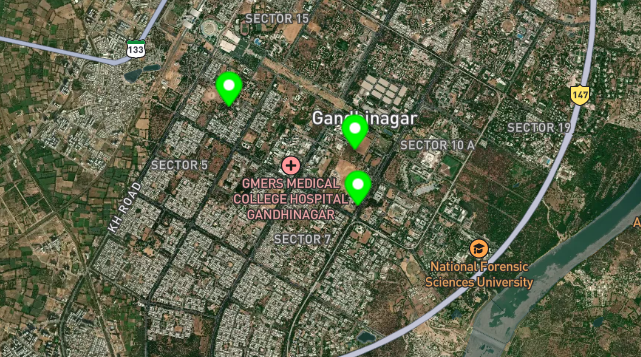
- Single coordinate pair
(x, y)— in geographic data usually (longitude, latitude) in that order (GeoJSON / WGS84). - Zero-length object: no area, no length; only position.
- Examples: cities, weather stations, GPS fixes, sampling sites.
Example GeoJSON (one Point feature with properties):
{
  "type": "Feature",
  "properties": {
    "name": "Trailhead Kiosk",
    "amenity": "information"
  },
  "geometry": {
    "type": "Point",
    "coordinates": [-122.4194, 37.7749]
  }
}
Lines (LineStrings)
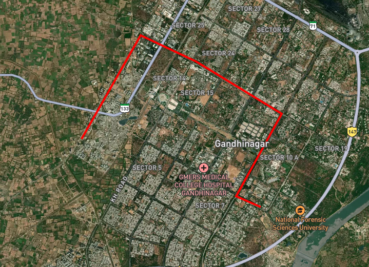
- Ordered sequence of vertices; the line connects them in order (no branching in a single
LineString). - Has length, no area.
- Examples: roads, rivers, trails, ship tracks.
Example GeoJSON (LineString with four vertices):
{
  "type": "Feature",
  "properties": {
    "name": "Ridge Trail segment",
    "surface": "unpaved"
  },
  "geometry": {
    "type": "LineString",
    "coordinates": [
      [-122.422, 37.773],
      [-122.418, 37.775],
      [-122.415, 37.7765],
      [-122.412, 37.778]
    ]
  }
}
Polygons
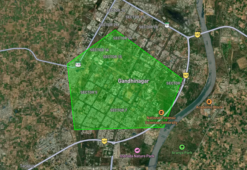
- Exterior ring is closed (first point equals last in valid data); interior rings (holes) are optional.
- Has area and perimeter (boundary length).
- Examples: countries, parcels, lakes, study regions.
Example GeoJSON (Polygon: outer ring only; note the repeated closing coordinate):
{
  "type": "Feature",
  "properties": {
    "name": "Study area boundary",
    "zone_code": "A-12"
  },
  "geometry": {
    "type": "Polygon",
    "coordinates": [
      [
        [-122.425, 37.772],
        [-122.408, 37.772],
        [-122.408, 37.781],
        [-122.425, 37.781],
        [-122.425, 37.772]
      ]
    ]
  }
}
Raster data in GIS
Vector data stores objects (points, lines, polygons) with coordinates and attributes. Raster data stores values on a regular grid of pixels (also called cells): each cell has a row/column index and usually one or more numeric values (bands). The grid is anchored in map space by origin, cell size (resolution), extent, and CRS—you will tie those ideas to CRS metadata in the next section.
How a raster differs from vector
| Vector | Raster | |
|---|---|---|
| Geometry | Exact vertices and edges | Uniform rectangles (pixels) |
| Best for | Boundaries, networks, discrete features | Continuous fields, imagery, scanned maps |
| Storage | Often smaller for sparse features | Can be large at fine resolution |
TIFF
TIFF (Tagged Image File Format) is a flexible image and raster container: “tags” in the file header describe image width and height, bits per sample, number of bands, compression (often none or LZW/deflate for GIS), and optional color maps. TIFF is widely used because it supports large files, lossless storage, and many bands—ideal for elevation models and satellite tiles.
When those tags include georeferencing (CRS, pixel size, origin), the file is usually called GeoTIFF. For a quick browser preview of a GeoTIFF you generated or downloaded, you can use tools such as the Pozyx Online GeoTIFF Viewer; Module 4 discusses limits and when to switch to QGIS or Python.
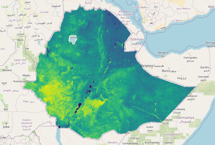 Pixels in a TIFF file are small grid cells, each storing a value representing color, intensity, or geographic data information.
![]()
Raster vocabulary
- Resolution — ground distance covered by one pixel edge (e.g. 10 m pixels).
- Extent / bounding box — outer limits of the raster in map coordinates.
- NoData — a sentinel value meaning “no observation here” (important for masks and mosaics).
Coordinate Reference Systems (CRS)
A CRS is the metadata that tells software how to interpret coordinate numbers (axes, units, Earth model, and—if projected—which map projection). Without it, values like −122.4194, 37.7749 are ambiguous (degrees vs meters, which origin). Layers and rasters carry CRS in their metadata (often an EPSG code) so every vertex or pixel lines up correctly on the map.
graph TD
    A[Earth] --> B[3D Sphere]
    B --> C[2D Map Projection]
    C --> D[Coordinate System]
    D --> E[Your Map]

    F[Common CRS] --> G[WGS84 - GPS coordinates]
    F --> H[Web Mercator - Web maps]
    F --> I[UTM - Local accuracy]
Geographic CRS
A Geographic Coordinate Reference System uses the Earth as a sphere (or ellipsoid).
Uses Latitude (lat) and Longitude (long)
Units are in degrees (°)
Example:
👉 (19.0760°, 72.8777°)
Projected CRS
A Projected Coordinate Reference System converts Earth into a flat map.
Uses X, Y coordinates
Units are in meters or feet
Example:
👉 (500000, 2100000)
Geographic vs projected
| Geographic CRS | Projected CRS | |
|---|---|---|
| Coordinates | Usually longitude and latitude in degrees | Easting / northing (or x/y) in meters (or feet) |
| Earth shape | Angles on a reference ellipsoid | A flat map plane |
| Examples | WGS 84 — EPSG:4326 | Web Mercator — EPSG:3857; UTM — e.g. EPSG:32610 |
| Typical use | GPS, GeoJSON, global exchange | Web basemaps, local distance/area in meters |
Lon/lat are simply the usual geographic coordinate form; in a projected CRS the same place has different numbers (large eastings/northings) until you transform back.
Datum and EPSG (short)
A datum ties your ellipsoid and origin to real surveys; changing datum can shift coordinates by meters. EPSG codes (registry maintained by IOGP) are shorthand for a full CRS definition—EPSG:4326, 3857, 32610, etc.—so GIS apps and libraries agree on one interpretation.
Reprojection vs assigning CRS
Reprojection = transform geometry from CRS A to CRS B; the location stays the same, the numbers change. Assigning a CRS = “these numbers already mean this system”—it does not recalculate coordinates. Mixing the two (or mis-tagging degrees as meters) corrupts maps.
Same point near San Francisco in different CRS (your software reproduces the values):
| CRS | EPSG | First coordinate | Second coordinate |
|---|---|---|---|
| WGS 84 (geographic) | 4326 | −122.4194° (lon) | 37.7749° (lat) |
| Pseudo-Mercator | 3857 | −13,627,665 m (easting) | 4,547,675 m (northing) |
| UTM zone 10N | 32610 | 551,131 m (easting) | 4,180,999 m (northing) |
Do not paste lon/lat into a layer declared as a meter CRS without a proper transform.
Typical problems (checklist)
- No CRS — software guesses or leaves the layer “unknown”; vectors/rasters fail to align with trusted data.
- Wrong tag — degrees labeled as 3857 (plots near null island); meters labeled as 4326 (stretched nonsense).
- Mixed CRS — overlay, buffer, join, and area need one common CRS (reproject first).
- Wrong tool for measure — distance/area in 4326 are in degrees / degree²; use a local projected CRS for meters/hectares when needed.
CRS workflow
- Record what CRS the coordinates actually use; assign metadata only when that is true.
- Reproject when you need a different CRS for analysis or display; align all layers before spatial join or merge.
Common Coordinate Reference Systems
| CRS | EPSG Code | Description | Use Case |
|---|---|---|---|
| WGS 84 | 4326 | Geographic lon/lat on WGS 84 | GPS, GeoJSON, interchange |
| Web Mercator | 3857 | x/y meters (web tiling) | Basemaps, slippy maps |
| UTM | Zone codes (e.g. 32610) | Metric bands | Local mapping, engineering |
Basic Assignments
1. City Population Analyzer
- Create a dictionary of cities with population and area
- Calculate population density using functions
- Find highest density city
- Export results to CSV using pandas
2. GeoJSON Feature Creator
- Create Point, LineString, and Polygon GeoJSON objects
- Store feature properties in dictionaries
- Print geometry types and coordinates
- Save GeoJSON data into a text file
3. Weather Data Processing
- Read temperature data from CSV using pandas
- Handle missing values
- Convert Celsius to Fahrenheit
- Find hottest and coldest days using loops
4. CRS Information Tool
- Create a dictionary of EPSG codes
- Compare Geographic CRS and Projected CRS
- Take user input for EPSG code
- Print CRS details using conditionals
5. Raster Metadata Simulator
- Create raster metadata dictionary
- Store width, height, bands, CRS, datatype
- Calculate total pixels using NumPy
- Identify raster type: continuous or categorical
6. File Handling and Coordinate Reader
- Create a text file containing city coordinates
- Read file using
with open() - Use
pathlibfor file paths - Print formatted coordinate information
7. GIS Data Type Classifier
- Ask user for GIS data type
- Identify vector or raster data
- Print suitable use cases
- Use
if,elif, and loops
8. NumPy Coordinate Calculator
- Store coordinates in NumPy arrays
- Calculate distance from origin
- Find minimum and maximum distances
- Perform vectorized calculations
9. Country Data Analysis using pandas
- Create DataFrame with country population, area, and GDP
- Calculate population density and GDP per capita
- Sort countries by GDP per capita
- Export final results to CSV
10. Mini GIS Explorer Project
- Read city data from CSV
- Store coordinates and attributes
- Create GeoJSON output
- Analyze data using pandas and NumPy
- Display CRS information for the dataset
Next Steps
In the next module, we'll dive deeper into vector analysis: - Working with GeoDataFrames - Spatial operations (buffers, intersections) - Attribute-based filtering - Spatial joins - Creating new geographic features
graph LR
    A[GIS Fundamentals] --> B[Vector Analysis]
    B --> C[Spatial Operations]
    B --> D[Attribute Queries]
    B --> E[Geometric Calculations]