Map Scale, Resolution, and Accuracy
Developing accurate water models requires understanding the quality, detail, and limits of spatial datasets. This section explains the concepts of map scale, spatial/temporal/spectral resolutions, the difference between accuracy and precision, and how scale dependency affects spatial analysis.
Presentation Slides
You can download or view the lecture slides for this topic: Map_scale_resolution.pdf
1. Map Scale
Map scale is the relationship between distance on the map and distance on the ground. It is expressed in three ways:
-
Representative Fraction (Ratio): e.g., \(1:50,000\) (meaning \(1\text{ cm}\) on the map equals \(50,000\text{ cm}\) or \(500\text{ m}\) on the ground).
-
Verbal Statement: e.g., "One centimeter represents 500 meters."
-
Graphic (Bar Scale): A scale bar drawn on the map layout that scales dynamically if the map is resized.
[!IMPORTANT] * Large-Scale Maps: Show a small geographic area in high detail (e.g., \(1:5,000\), showing building footprints and town drainage ditches). * Small-Scale Maps: Show a large geographic area with less detail (e.g., \(1:1,000,000\), showing national borders and primary river basins).
2. Spatial, Temporal, Spectral, and Radiometric Resolutions
In remote sensing and raster modeling, resolution determines the level of detail captured:
graph TD
    Res["Image Resolution"] --> Spat["1. Spatial"]
    Res --> Temp["2. Temporal"]
    Res --> Spec["3. Spectral"]
    Res --> Rad["4. Radiometric"]

    Spat --> Spat_D["Ground Pixel Size<br/>e.g., Sentinel-2 (10m),<br/>Landsat (30m)"]
    Temp --> Temp_D["Revisit Time<br/>e.g., Sentinel-2 (5 days),<br/>MODIS (daily)"]
    Spec --> Spec_D["Light Bands<br/>e.g., Sentinel-2 (12 bands)"]
    Rad --> Rad_D["Bit Depth (Sensors)<br/>e.g., 8-bit (256 values),<br/>12-bit (4096 values)"]
Applications in Hydrology:
-
Spatial: A \(90\text{ m}\) elevation raster is too coarse to detect narrow mountain gullies, which can lead to errors in stream network calculation. A \(12.5\text{ m}\) DEM is much more effective for modeling terrain at this scale.
-
Temporal: Flood mapping requires high temporal resolution (daily or sub-daily observations) to capture the peak water level. Drought monitoring can use lower temporal resolutions (e.g., 8-day or monthly composite datasets).
-
Spectral: Multi-spectral bands are needed to calculate indexes like the Normalized Difference Water Index (NDWI), which isolates water bodies by comparing green light reflection with shortwave infrared absorption.
-
Radiometric: Higher bit depth (e.g., Landsat 8/9's 12-bit or Sentinel-2's 12-bit data) increases the sensor's sensitivity to subtle differences in reflected energy. This is critical when monitoring water quality parameters like turbidity, suspended sediment concentrations, or chlorophyll-a, where water surface reflectance values are extremely low.
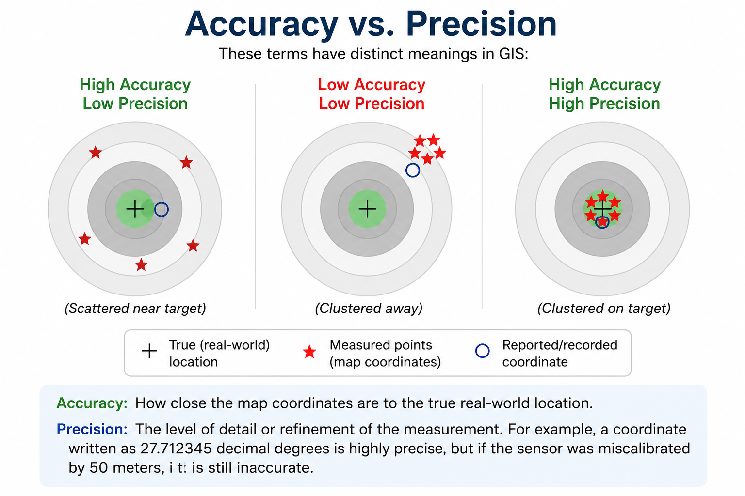
3. Accuracy vs. Precision
These terms have distinct meanings in GIS:
-
Accuracy: How close the map coordinates are to the true real-world location.
-
Precision: The level of detail or refinement of the measurement. For example, a coordinate written as
27.712345decimal degrees is highly precise, but if the sensor was miscalibrated by 50 meters, it is still inaccurate.
Vertical Accuracy in Hydrology (\(LE_{90}\) and \(RMSE_z\))
While horizontal accuracy defines the location of boundaries, vertical accuracy (\(Z\)-coordinate) is far more critical in water resource engineering and hydrological modeling.
- \(LE_{90}\) (Linear Error at 90% Confidence): A metric indicating that 90% of vertical elevations in a dataset are within a specified distance of their true value.
- \(RMSE_z\) (Root Mean Square Error in Z): The standard deviation of the difference between dataset elevations and reference checkpoints.
- Hydrological Impact: In flat floodplains, a vertical error of just \(0.5\text{ m}\) in a DEM can result in kilometers of difference in predicted flood inundation boundaries.
4. Scale Dependency and Generalization
Geospatial features change their representation depending on the scale of the map:
-
Vector Generalization: At \(1:5,000\), a river bank is mapped as a detailed polygon showing sandbars and bends. At \(1:1,000,000\), the same river is simplified to a single line, smoothing out small curves.
-
The Coastline Paradox: The measured length of a river changes depending on the measurement scale. Large-scale maps capture small channel bends, resulting in a longer total stream length calculation than small-scale maps where these curves are smoothed out.
[!TIP] When compiling spatial data for a project, ensure that all layers are mapped at a similar scale to prevent topological misalignment during overlay analysis.
5. Error Propagation in Hydrological Models
When spatial datasets containing minor inaccuracies are used in secondary calculations, those errors multiply. This process is called error propagation:
flowchart TD
    RawDEM["1. Raw DEM<br/>(Contains minor vertical <br/>errors/sinks)"] -->|Sink Fill Algorithm| FilledDEM["2. Filled DEM<br/>(Modified elevations<br/> to enforce drainage)"]
    FilledDEM -->|D8 / D-Infinity| FlowDir["3. Flow Direction<br/>(Skewed cell directions due <br/>to filled sinks)"]
    FlowDir -->|Flow Accumulation| FlowAcc["4. Flow Accumulation<br/>(Mislocated stream channels <br/>& basin divides)"]
    FlowAcc -->|Hydrograph Modeling| Runoff["5. Runoff Hydrograph<br/>(Inaccurate peak timing and <br/>volume forecasts)"]

    style RawDEM fill:#f9d5d5,stroke:#c0392b,stroke-width:2px
style Runoff fill:#f9e79f,stroke:#d4ac0d,stroke-width:2px- Sink Filling Artifacts: DEMs contain natural depressions, but also artificial ones caused by sensor noise. Hydrological tools must "fill" these artificial sinks to allow continuous flow routing. If a DEM is coarse or has poor vertical accuracy, massive depressions are artificially filled, flattening real valleys and altering the calculated flow path directions.
- Mislocated Divides: A tiny vertical deviation on a ridge line can cause the D8 routing algorithm to route runoff into an adjacent sub-basin, incorrectly calculating the total drainage area of the watershed.
6. Resampling Impacts on Continuous Grids
Resampling is necessary when combining layers of different resolutions (e.g., matching a \(30\text{ m}\) Landsat precipitation grid with a \(10\text{ m}\) Sentinel-2 land cover map). However, the chosen resampling method directly alters data integrity:
-
Nearest Neighbor:
- How it works: Assigns the value of the nearest cell without interpolation.
- Hydrological Impact: Best for categorical data (e.g., LULC classes, soil types) as it preserves discrete values. Avoid for DEMs and precipitation, as it creates jagged, step-like artifacts along terrain slopes.
- Risk: Can cause artificial flow disconnections or blockages in narrow valleys.
-
Bilinear Interpolation / Cubic Convolution:
- How it works: Computes a distance-weighted average of neighboring cells (\(4\) for Bilinear, \(16\) for Cubic).
- Hydrological Impact: Ideal for continuous datasets like elevation and temperature. It produces smooth slope grids, which are essential for calculating realistic hydraulic gradients and hydrological routing.
- Risk: Never use on land-use classifications (e.g., averaging Land Use Class 3 (Water) and Class 5 (Urban) results in Class 4, which is physically meaningless).